Outside Surface Heat Balance[LINK]

The heat balance on the outside face is:

where:

~~= Absorbed direct and diffuse solar (short wavelength) radiation heat flux.

~~= Net long wavelength (thermal) radiation flux exchange with the air and surroundings.

~~= Convective flux exchange with outside air.

~~= Conduction heat flux (q/A) into the wall.

All terms are positive for net flux to the face except the conduction term, which is traditionally taken to be positive in the direction from outside to inside of the wall. Simplified procedures generally combine the first three terms by using the concept of a sol-air temperature. Each of these heat balance components is introduced briefly below.

External Shortwave Radiation[LINK]

~~ is calculated using procedures presented later in this manual and includes both direct and diffuse incident solar radiation absorbed by the surface face. This is influenced by location, surface facing angle and tilt, surface face material properties, weather conditions, etc.

External Longwave Radiation[LINK]

is a standard radiation exchange formulation between the surface, the sky, and the ground. The radiation heat flux is calculated from the surface absorptivity, surface temperature, sky and ground temperatures, and sky and ground view factors.

The longwave radiation heat exchange between surfaces is dependent on surface temperatures, spatial relationships between surfaces and surroundings, and material properties of the surfaces. The relevant material properties of the surface, emissivity and absorptivity , are complex functions of temperature, angle, and wavelength for each participating surface. However, it is generally agreed that reasonable assumptions for building loads calculations are (Chapman 1984; Lienhard 1981):

each surface emits or reflects diffusely and is gray and opaque ( = , = 0, = 1- )

each surface is at a uniform temperature

energy flux leaving a surface is evenly distributed across the surface,

the medium within the enclosure is non-participating.

These assumptions are frequently used in all but the most critical engineering applications.

Table: Nomenclature List of Variables.

Mathematical variable|Description|UnitsRange ———————|———–|———- q”_LWR|Exterior surface longwave radiation flux|W/m²|- h_r|Linearized radiative heat transfer coefficient to air temperature|W/(m² K)|- T_surf|Surface Outside face temperatures |K|- T_air|Outside air temperature|K|- T_gnd||Environmental ground surface temperature|K|- T_sky|Sky Effective temperature |K|- F_gnd|view factor of wall surface to ground surface|-|0~1\ F~sky~|View factor of wall surface to sky|-|0~1\ F~air~|View factor of wall surface to air|-|0~1 |Surface long-wave emissivity |-|0~1 |Stefan-Boltzmann constant|W/m²-K⁴|0.0000000567

Consider an enclosure consisting of building exterior surface, surrounding ground surface, and sky. Using the assumptions above, we can determine the longwave radiative heat flux at the building exterior surface (Walton 1983; McClellan and Pedersen 1997). The total longwave radiative heat flux is the sum of components due to radiation exchange with the ground, sky, and air.

Applying the Stefan-Boltzmann Law to each component yields:

where

 =long-wave emittance of the surface

 =Stefan-Boltzmann constant

F_gnd = view factor of wall surface to ground surface temperature

F_sky = view factor of wall surface to sky temperature

F_air =view factor of wall surface to air temperature

T_surf = outside surface temperature

T_gnd = ground surface temperature

T_sky = sky temperature

T_air = air temperature

Linearized radiative heat transfer coefficients are introduced to render the above equation more compatible with the heat balance formulation,

where

The longwave view factors to ground and sky are calculated with the following expressions (Walton 1983):

where  is the tilt angle of the surface. The view factor to the sky is further split between sky and air radiation by:

The ground surface temperature is assumed to be the same as the air temperature. The final forms of the radiative heat transfer coefficients are shown here.

References[LINK]

ASHRAE. 1993. 1993 ASHRAE Handbook – Fundamentals. Atlanta: American Society of Heating, Refrigerating, and Air-Conditioning Engineers, Inc.

Chapman, A. J. 1984. Heat Transfer, 4^th Edition, New York: Macmillan Publishing Company.

Lienhard, J. H. 1981. A Heat Transfer Textbook, Englewood Cliffs, N.J.: Prentice-Hall, Inc.

McClellan, T. M., and C. O. Pedersen. 1997. Investigation of Outside Heat Balance Models for Use in a Heat Balance Cooling Load Calculation. ASHRAE Transactions, Vol. 103, Part 2, pp. 469-484.

Walton, G. N. 1983. Thermal Analysis Research Program Reference Manual. NBSSIR 83-2655. National Bureau of Standards.

Atmospheric Variation[LINK]

All buildings are located in the troposphere, the lowest layer of the atmosphere. The troposphere extends from sea level to an altitude of 11 km. Throughout the troposphere, air temperature decreases almost linearly with altitude at a rate of approximately 1°C per 150 m. Barometric pressure decreases more slowly. Wind speed, on the other hand, increases with altitude.

Because the atmosphere changes with altitude (defined as height above ground in this case), tall buildings can experience significant differences in local atmospheric properties between the ground floor and the top floor. Buildings interact with the atmosphere through convective heat transfer between the outdoor air and the exterior surfaces of the building envelope, and through the exchange of air between the outside and inside of the building via infiltration and ventilation.

Impetus for using this modeling is illustrated in the next table. Using a 70 story (284 meters) building as an example, the atmospheric variables are significant.

Atmospheric Variables at Two Different Altitudes above Ground Level

Variable	1.5 Meters	284 meters	Absolute Diff	Percent Diff
Air Temperature	15°C	13.15°C	1.85°C	12.3%
Barometric Pressure	101,325 Pa	97,960 Pa	3,365 Pa	3.3%
Wind Speed	2.46 m/s	7.75 m/s	5.29 m/s	215%

Comparing the annual energy usage between 60 discretely modeled floors of a building, it turns out that the effect due to wind speed change is dominant over the first ten floors. But at floor 25, surprisingly, the effect due to air temperature has caught up and is about equal to the effect of wind speed. Above floor 25 the effect due to air temperature is now dominant. Clearly it is desirable to model air temperature variation with altitude for high-rise buildings.

To accommodate atmospheric variation EnergyPlus automatically calculates the local outdoor air temperature and wind speed separately for each zone and surface that is exposed to the outdoor environment. The zone centroid or surface centroid are used to determine the height above ground. Only local outdoor air temperature and wind speed are currently calculated because they are important factors for the exterior convection calculation for surfaces (see Exterior Convection below) and can also be factors in the zone infiltration and ventilation calculations. Variation in barometric pressure, however, is considered when using the Airflow Network objects.

Local Outdoor Air Temperature Calculation[LINK]

Variation in outdoor air temperature is calculated using the U.S. Standard Atmosphere (1976). According to this model, the relationship between air temperature and altitude in a given layer of the atmosphere is:

where

T_z = air temperature at altitude z

T_b = air temperature at the base of the layer, i.e., ground level for the troposphere

L = air temperature gradient, equal to –0.0065 K/m in the troposphere

H_b = offset equal to zero for the troposphere

H_z = geopotential altitude.

The variable H_z is defined by:

where

E = 6,356 km, the radius of the Earth

z = altitude.

For the purpose of modeling buildings in the troposphere, altitude z refers to the height above ground level, not the height above sea level. The height above ground is calculated as the height of the centroid, or area-weighted center point, for each zone and surface.

The air temperature at ground level, T_b, is derived from the weather file air temperature by inverting the equation above:

where

T_z,met = weather file air temperature (measured at the meteorological station)

z_met = height above ground of the air temperature sensor at the meteorological station.

The default value for z_met for air temperature measurement is 1.5 m above ground. This value can be overridden by using the Site:WeatherStation object.

Local Wind Speed Calculation[LINK]

Chapter 16 of the Handbook of Fundamentals (ASHRAE 2005). The wind speed measured at a meteorological station is extrapolated to other altitudes with the equation:

where

z = altitude, height above ground

V_z = wind speed at altitude z

 = wind speed profile exponent at the site

 = wind speed profile boundary layer thickness at the site

z_met = height above ground of the wind speed sensor at the meteorological station

V_met = wind speed measured at the meteorological station

_met = wind speed profile exponent at the meteorological station

_met = wind speed profile boundary layer thickness at the meteorological station.

The wind speed profile coefficients , , _met, and _met, are variables that depend on the roughness characteristics of the surrounding terrain. Typical values for  and  are shown in the following table:

Wind Speed Profile Coefficients (ASHRAE Fundamentals 2005).

Terrain Description	Exponent, 	Boundary Layer Thickness,  (m)
Flat, open country	0.14	270
Rough, wooded country	0.22	370
Towns and cities	0.33	460
Ocean	0.10	210
Urban, industrial, forest	0.22	370

The terrain types above map to the options in the Terrain field of the Building object. The Terrain field can be overridden with specific values for  and  by using the Site:HeightVariation object.

The default value for z_met for wind speed measurement is 10 m above ground. The default values for _met and _met are 0.14 and 270 m, respectively, because most meteorological stations are located in an open field. These values can be overridden by using the Site:WeatherStation object.

Outdoor/Exterior Convection[LINK]

Heat transfer from surface convection is modeled using the classical formulation:

where

Q_c = rate of exterior convective heat transfer

h_c,ext = exterior convection coefficient

A = surface area

T_surf = surface temperature

T_air = outdoor air temperature

Substantial research has gone into the formulation of models for estimating the exterior convection coefficient. Since the 1930’s there have been many different methods published for calculating this coefficient, with much disparity between them (Cole and Sturrock 1977; Yazdanian and Klems 1994). More recently Palyvos (2008) surveyed correlations cataloging some 91 different correlations into four categories based on functional form of the model equation. EnergyPlus therefore offers a wide selection of different methods for determining values for h_c,ext. The selection of model equations for h_c,extcan be made at two different levels. The first is the set of options available in the input object SurfaceConvectionAlgorithm:Outside that provides a way of broadly selecting which model equations are applied throughout the model. The input objects SurfaceProperty:ConvectionCoefficients and SurfaceProperty:ConvectionCoefficients:MultipleSurface also provide ways of selecting which model equations or values are applied for specific surfaces. These basic options are identified by the key used for input and include:

SimpleCombined

TARP

MoWiTT

DOE-2

AdaptiveConvectionAlgorithm

Note that when the outside environment indicates that it is raining, the exterior surfaces (exposed to wind) are assumed to be wet. The convection coefficient is set to a very high number (1000) and the outside temperature used for the surface will be the wet-bulb temperature. (If you choose to report this variable, you will see 1000 as its value.)

When the AdaptiveConvectionAlgorithm is used, there is a second, deeper level of control available for selecting among a larger variety of h_c,ext equations and also defining custom equations using curve or table objects. These options are described in this section.

In addition to the correlation choices described below, it is also possible to override the convection coefficients on the outside of any surface by other means:

• Use the SurfaceProperty:ConvectionCoefficients object in the input file to set the convection coefficient value on either side of any surface.
• Use the SurfaceProperty:OtherSideCoefficients object in the input file to set heat transfer coefficients and temperatures on surfaces.
• Use the EnergyManagementSystem Actuators that are available for overriding h_c values.
• These options can also use schedules to control values over time. Specific details are given in the Input Output Reference document.

Simple Combined[LINK]

The simple algorithm uses surface roughness and local surface windspeed to calculate the exterior heat transfer coefficient (key:SimpleCombined). The basic equation used is:

where

h = heat transfer coefficient

V_z = local wind speed calculated at the height above ground of the surface centroid

D, E, F = material roughness coefficients

The roughness correlation is taken from Figure 1, Page 22.4, ASHRAE Handbook of Fundamentals (ASHRAE 1989). The roughness coefficients are shown in the following table:

Roughness Coefficients D, E, and F.

Roughness Index	D	E	F	Example Material
1 (Very Rough)	11.58	5.894	0.0	Stucco
2 (Rough)	12.49	4.065	0.028	Brick
3 (Medium Rough)	10.79	4.192	0.0	Concrete
4 (Medium Smooth)	8.23	4.0	-0.057	Clear pine
5 (Smooth)	10.22	3.1	0.0	Smooth Plaster
6 (Very Smooth)	8.23	3.33	-0.036	Glass

Note that the simple correlation yields a combined convection and radiation heat transfer coefficient. Radiation to sky, ground, and air is included in the exterior convection coefficient for this algorithm.

All other algorithms yield a convection only heat transfer coefficient. Radiation to sky, ground, and air is calculated automatically by the program.

TARP ALGORITHM[LINK]

TARP, or Thermal Analysis Research Program, is an important predecessor of EnergyPlus (Walton 1983). Walton developed a comprehensive model for exterior convection by blending correlations from ASHRAE and flat plate experiments by Sparrow et. al. In older versions of EnergyPlus, prior to version 6, the “TARP” model was called “Detailed.” The model was reimplemented in version 6 to use Area and Perimeter values for the group of surfaces that make up a facade or roof, rather than the single surface being modeled.

Nomenclature List of Variables.

Variable

Description

Units

Range

A

Surface area of the surface

m²

/= 0

h_c

Surface exterior convective heat transfer coefficient

W/(m²K)

h_f

Forced convective heat transfer coefficient

W/(m²K)

h_n

Natural convective heat transfer coefficient

W/(m²K)

P

Perimeter of surface

m

R_f

Surface roughness multiplier

T_air

Local outdoor air temperature calculated at the height above ground of the surface centroid

C

T_so

Outside surface temperature

C

T

Temperature difference between the surface and air,

C

V_z

Local wind speed calculated at the height above ground of the surface centroid

m/s

W_f

Wind direction modifier

Angle between the ground outward normal and the surface outward normal

degree

Roughness Index

Surface roughness index (6=very smooth, 5=smooth, 4=medium smooth, 3=medium rough, 2=rough, 1=very rough)

1~6

The Detailed, BLAST, and TARP convection models are very similar. In all three models, convection is split into forced and natural components (Walton 1981). The total convection coefficient is the sum of these components.

The forced convection component is based on a correlation by Sparrow, Ramsey, and Mass (1979):

where

W_f = 1.0 for windward surfaces

or

W_f = 0.5 for leeward surfaces

Leeward is defined as greater than 100 degrees from normal incidence (Walton 1981).

The surface roughness multiplier Rf is based on the ASHRAE graph of surface conductance (ASHRAE 1981) and may be obtained from the following table:

Surface Roughness Multipliers (Walton 1981).

Roughness Index	Rf	Example Material
1 (Very Rough)	2.17	Stucco
2 (Rough)	1.67	Brick
3 (Medium Rough)	1.52	Concrete
4 (Medium Smooth)	1.13	Clear pine
5 (Smooth)	1.11	Smooth Plaster
6 (Very Smooth)	1.00	Glass

The natural convection component h_n is calculated in the same way as the interior “Detailed” model. The detailed natural convection model correlates the convective heat transfer coefficient to the surface orientation and the difference between the surface and zone air temperatures (where T = Air Temperature - Surface Temperature). The algorithm is taken directly from Walton (1983). Walton derived his algorithm from the ASHRAE Handbook (2001), Table 5 on p. 3.12, which gives equations for natural convection heat transfer coefficients in the turbulent range for large, vertical plates and for large, horizontal plates facing upward when heated (or downward when cooled). A note in the text also gives an approximation for large, horizontal plates facing downward when heated (or upward when cooled) recommending that it should be half of the facing upward value. Walton adds a curve fit as a function of the cosine of the tilt angle to provide intermediate values between vertical and horizontal. The curve fit values at the extremes match the ASHRAE values very well.

For no temperature difference OR a vertical surface the following correlation is used:

For (T < 0.0 AND an upward facing surface) OR (T > 0.0 AND an downward facing surface) an enhanced convection correlation is used:

where  is the surface tilt angle.

For (T > 0.0 AND an upward facing surface) OR (T < 0.0 AND an downward facing surface) a reduced convection correlation is used:

where  is the surface tilt angle.

MoWiTT Algorithm[LINK]

Nomenclature List of Variables.

Variable	Description	UnitsRange
A	Constant	W/(m2K(m/s)b
B	Constant	-
Ct	Turbulent natural convection constant	W/(m2K4/3)
hc	Surface exterior convective heat transfer coefficient	W/(m2K)
Tso	Outside surface temperature	C/K
T	Temperature difference between the surface and air	C/K

The MoWiTT model is based on measurements taken at the Mobile Window Thermal Test (MoWiTT) facility (Yazdanian and Klems 1994). The correlation applies to very smooth, vertical surfaces (e.g. window glass) in low-rise buildings and has the form:

Constants a, b and turbulent natural convection constant C_t are given in Table 10. The original MoWiTT model has been modified for use in EnergyPlus so that it is sensitive to the local suface’s wind speed which varies with the height above ground. The original MoWiTT model was formulated for use with the air velocity at the location of the weather station. As of Version 7.2, EnergyPlus uses the “a” model coefficients derived by Booten et al. (2012) rather than the original values from Yazdanian and Klems (1994).

NOTE: The MoWiTT algorithm may not be appropriate for rough surfaces, high-rise surfaces, or surfaces that employ movable insulation.

MoWiTT Coefficients (Yazdanian and Klems 1994, Booten et al. 2012)

Wind Direction	Ct	a	b
(Units)	W/m2K4/3	W/m2K(m/s)b	-
Windward	0.84	3.26	0.89
Leeward	0.84	3.55	0.617

DOE-2 Model[LINK]

Nomenclature List of Variables.

Variable	Description	UnitsRange
a	Constant	W/(m2K(m/s)b
b	Constant	-
hc	Surface exterior convective heat transfer coefficient	W/(m2K)
hc,glass	Convective heat transfer coefficient for very smooth surfaces (glass)	W/(m2K)
hn	Natural convective heat transfer coefficient	W/(m2K)
Rf	Surface roughness multiplier	-
Tso	Outside surface temperature	C/K
T	Temperature difference between the surface and air,	C/K
Angle between the ground outward normal and the surface outward normal	radian	-

The DOE-2 convection model is a combination of the MoWiTT and BLAST Detailed convection models (LBL 1994). The convection coefficient for very smooth surfaces (e.g. glass) is calculated as:

h_n is calculated using Equation or Equation . Constants a and b are given in Table 10.

For less smooth surfaces, the convection coefficient is modified according to the equation

where R_f is the roughness multiplier given by Table 8.

Adaptive Convection Algorithm[LINK]

This algorithm has a structure that allows for finer control over the models used for particular surfaces. The algorithm for the outside face was developed for EnergyPlus but it borrows concepts and its name from the research done by Beausoleil-Morrison (2000, 2002) for convection at the inside face (see the description below for interior convection).

The adaptive convection algorithm implemented in EnergyPlus for the outside face is much simpler than that for the inside face. The surface classification system has a total of 4 different categories for surfaces that depend on current wind direction and heat flow directions. However it is more complex in that the h_c equation is split into two parts and there are separate model equation selections for forced convection, h_f, and natural convection, h_n. The following table summarizes the categories and the default assignments for h_c equations. The individual h_c equations are documented below.

Adaptive Convection Algorithm Details

Surface Classifi-cation

Heat FlowDirection

Wind Direct-ion

h_f Models

h_n~~Models

1

Roof Stable

Down

Any

TARPWindwardMoWiTTWindwardDOE2WindwardNusseltJurgesBlockenWindwardEmmelRoofClearRoof

WaltonStableHorizontalOrTiltAlamdariStableHorizontal

2

Roof Unstable

Up

Any

TARPWindwardMoWiTTWindwardDOE2WindwardNusseltJurgesBlockenWindwardEmmelRoofClearRoof

WaltonUnstableHorizontalOrTiltAlamdariUnstableHorizontal

3

Vertical Wall Windward

Any

Windward

TARPWindwardDOE2WindwardMoWiTTWindwardNusseltJurgesMcAdamsMitchellBlockenWindwardEmmelVertical

ASHRAEVerticalWallAlamdariHammondVerticalWallFohannoPolidoriVerticalWallISO15099Windows

4

Vertical Wall Leeward

Any

Leeward

TARPLeewardMoWiTTLeewardDOE2LeewardEmmelVerticalNusseltJurgesMcAdamsMitchell

ASHRAEVerticalWallAlamdariHammondVerticalWallFohannoPolidoriVerticalWallISO15099Windows

Outside Face Surface Classification[LINK]

During an initial setup phase, all the heat transfer surfaces in the input file are analyzed in groups to determine appropriate values for geometry scales used in many of the convection correlations. Eight separate groups are assembled for nominally vertical exterior surfaces for eight bins of azimuth: north, northeast, east, southeast, south, southwest, west, northwest. Surfaces with the same range of azimuth are grouped together and analyzed for overall geometry parameters. A ninth group is assembled for nominally horizontal exterior surfaces for a roof bin that is also analyzed for geometry. These geometry routines find bounds and limits of all the surfaces in the group and then model geometric parameters from these limits.

Sparrow Windward[LINK]

As discussed above for the TARP algorithm, a Sparrow et al. (1979) conducted flat plate measurements and develop the following correlation for finite-size flat plates oriented to windward.

Sparrow Leeward[LINK]

Sparrow et al. (1979) conducted flat plate measurements and develop the following correlation for finite-size flat plates oriented to leeward.

MoWITT Windward[LINK]

As discussed above, Yazdanian and Klems (1994) used outdoor laboratory measurements to develop the following correlation for smooth surfaces oriented to windward. Booten et al. (2012) developed revised coefficients for use with local surface wind speeds.

This model equation is for the total film coefficient and includes the natural convection portion. Therefore it should not be used in conjunction with a second natural convection model equation.

MoWITT Leeward[LINK]

Yazdanian and Klems (1994) used outdoor laboratory measurements to develop the following correlation for smooth surfaces oriented to leeward. Booten et al. (2012) developed revised coefficients for use with local surface wind speeds.

This model equation is for the total film coefficient and includes the natural convection portion. Therefore it should not be used in conjunction with a second natural convection model equation.

Blocken[LINK]

Blocken et al. (2009) developed a set of correlations for windward facing outdoor surfaces using numerical methods (key: BlockenWindward).

Where V_10m is the air velocity at the location of the weather station and θ is the angle of incidence between the wind and the surface in degrees. This model is only applicable to windward surfaces and lacks a natural convection component and therefore cannot be used on its own but only within the adaptive convection algorithm for the outside face.

Clear[LINK]

Clear et al. (2003) developed correlations from measurements for horizontal roofs on two commercial buildings. In EnergyPlus the implementation uses the model for natural convection plus turbulent forced convection (eq. 8A in the reference) and applies it to the center point of each surface section that makes up the roof.

Where

x is the distance to the surface centroid from where the wind begins to intersect the roof. In EnergyPlus this is currently simplified to half the square root of the roof surface.

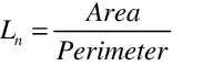of overall roof

is the thermal conductivity of air

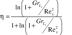is the weighting factor for natural convection (suppressed at high forced convection rates)

is the Rayleigh number

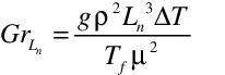is the Grashof number

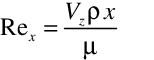is the Reynolds number at x

Pr is the Prandtl number

This model only claims to be applicable to horizontal roof surfaces so it may not be applicable to tilted roofs. It combines natural and forced convection and therefore should not be used in conjunction with yet another natural convection model.

Emmel[LINK]

Emmel et al. (2007) developed a set of correlations for outdoor surfaces using numerical methods. The following equations are for vertical surfaces (key: EmmelVertical):

Where V_10m is the air velocity at the location of the weather station and θ is the angle of incidence between the wind and the surface in degrees. The following equations are used for horizontal (roof) surfaces (key: EmmelRoof):

Where θ is the angle of incidence between the wind and the longest edge of the roof surface in degrees.

This model is for all wind directions but lacks a natural convection component. The model was developed for simple, rectangular low-rise buildings. It is available only within the adaptive convection algorithm for the outside face

Nusselt Jurges[LINK]

Perhaps the oldest equation for wind-driven convection was developed by Nusselt and Jurges (1922). Palyvos (2008) casts their model in simplified form in SI units as:

Where V_z is the wind velocity in m/s, in EnergyPlus that velocity is adjusted for height above ground using the z axis coordinate of the surface’s centroid and the site wind model. This model can be applied to all surfaces and the relatively large constant is assumed to represent the natural convection portion of a total convection coefficient. The model is not sensitive to wind direction nor surface roughness.

McAdams[LINK]

A venerable equation for wind-driven convection was developed by McAdams (1954) which Palyvos (2008) casts in SI units as:

Where V_z is the wind velocity in m/s that has been adjusted for height above ground using the z axis coordinate of the surface’s centroid. This model can be applied to all surfaces and the relatively large constant is assumed to represent the natural convection portion of a total convection coefficient. The model is not sensitive to wind direction nor surface roughness.

Mitchell[LINK]

A useful geometric scale based on building volume is used in an equation developed by Mitchell (1976). The wind-driven convection equation is cast by Palyvos as:

Where V_z is the wind velocity in m/s that has been adjusted for height above ground using the z axis coordinate of the surface’s centroid and L is the cube root of the building’s total volume. EnergyPlus interprets this as the sum of the volume of all the zones in the input file.

Exterior/External Conduction[LINK]

The conduction term, _, can in theory be calculated using a wide variety of heat conduction formulations. Typically in EnergyPlus, the Conduction Transfer Function (CTF) method is used. The available models are described in this section: Conduction Through The Walls.

References[LINK]

ASHRAE. 1981. 1981 ASHRAE Handbook – Fundamentals, Atlanta: American Society of Heating, Refrigerating, and Air-Conditioning Engineers, Inc.

ASHRAE. 1989. 1989 ASHRAE Handbook – Fundamentals, Atlanta: American Society of Heating, Refrigerating, and Air-Conditioning Engineers, Inc.

ASHRAE. 1993. 1993 ASHRAE Handbook – Fundamentals, Chapter 3, Heat Transfer, I-P & S-I Editions, Atlanta: American Society of Heating, Refrigerating, and Air-Conditioning Engineers, Inc.

ASHRAE. 2001. 2001 ASHRAE Handbook – Fundamentals, Atlanta: American Society of Heating, Refrigerating, and Air-Conditioning Engineers, Inc.

ASHRAE. 2005. 2005 ASHRAE Handbook – Fundamentals, Chapter 16, Air Flow Around Buildings, Atlanta: American Society of Heating, Refrigerating, and Air-Conditioning Engineers, Inc.

Booten, C., N. Kruis, and C. Christensen. 2012. Identifying and Resolving Issues in EnergyPlus and DOE-2 Window Heat Transfer Calculations. National Renewable Energy Laboratory. NREL/TP-5500-55787. Golden, CO.

Cole, R. J., and N. S. Sturrock. 1977. The Convective Heat Exchange at the External Surface of Buildings. Building and Environment, Vol. 12, p. 207.

Ellis, P.G., and P.A. Torcellini. 2005. “Simulating Tall Buildings Using EnergyPlus”, Proceedings of the Ninth International IBPSA Conference, Building Simulation 2005, Montreal, Canada, August 15-18, 2005.

Lawrence Berkeley Laboratory (LBL). 1994. DOE2.1E-053 source code.

Sparrow, E. M., J. W. Ramsey, and E. A. Mass. 1979. Effect of Finite Width on Heat Transfer and Fluid Flow about an Inclined Rectangular Plate. Journal of Heat Transfer, Vol. 101, p. 204.

U.S. Standard Atmosphere. 1976. U.S. Government Printing Office, Washington, D.C.

Walton, G. N. 1981. Passive Solar Extension of the Building Loads Analysis and System Thermodynamics (BLAST) Program, Technical Report, United States Army Construction Engineering Research Laboratory, Champaign, IL.

Walton, G. N. 1983. Thermal Analysis Research Program Reference Manual. NBSSIR 83-2655. National Bureau of Standards.

Yazdanian, M. and J. H. Klems. 1994. Measurement of the Exterior Convective Film Coefficient for Windows in Low-Rise Buildings. ASHRAE Transactions, Vol. 100, Part 1, p. 1087.