Absorption Chiller[LINK]
The input object Chiller:Absorption
provides a model for absorption chillers that is an empirical
model of a standard absorption refrigeration cycle. The
condenser and evaporator are similar to that of a standard
chiller, which are both water-to-water heat exchangers. The
assembly of a generator and absorber provides the compression
operation. Low-pressure vapor from the evaporator is absorbed
by the liquid solution in the absorber. A pump receives
low-pressure liquid from the absorber, elevates the pressure
of the liquid, and delivers the liquid to the generator. In
the generator, heat from a high temperature source (hot water
or steam) drives off the vapor that has been absorbed by the
solution. The liquid solution returns to the absorber through
a throttling valve whose purpose is to provide a pressure drop
to maintain the pressure difference between the generator and
absorber. The heat supplied to the absorber can be waste heat
from a diesel jacket, or the exhaust heat from diesel, gas,
and steam turbines. For more information on absorption
chillers, see the Input/Output Reference Document (Object:
Chiller:Absorption).
The part-load ratio of the absoprtion chiller’s evaporator
is simply the actual cooling effect produced by the chiller
divided by the maximum cooling effect available.
where
 = part-load ratio of
chiller evaporator
= part-load ratio of
chiller evaporator
 = chiller evaporator load
[W]
= chiller evaporator load
[W]
 = rated chiller
evaporator capacity [W]
= rated chiller
evaporator capacity [W]
This absorption chiller model is based on a polynomial fit
of absorber performance data. The Generator Heat Input Part
Load Ratio Curve is a quadratic equation that determines the
ratio of the generator heat input to the demand on
the chiller’s evaporator (Qevap).
The Pump Electric Use Part Load Ratio Curve is a quadratic
equation that determines the ratio of the actual absorber
pumping power to the nominal pumping power.
Thus, the coefficient sets establish the ratio of heat
power in-to-cooling effect produced as a function of part load
ratio. The ratio of heat-power-in to cooling-effect-produced
is the inverse of the coefficient of performance.
If the operating part-load ratio is greater than the
minimum part-load ratio, the chiller will run the entire time
step and cycling will not occur (i.e. CyclingFrac =
1). If the operating part-load ratio is less than the minimum
part-load ratio, the chiller will be on for a fraction of the
time step equal to CyclingFrac. Steam (or hot water)
and pump electrical energy use are also calculated using the
chiller part-load cycling fraction.
where
 = chiller part-load
cycling fraction
= chiller part-load
cycling fraction
 = chiller minimum
part-load ratio
= chiller minimum
part-load ratio
 = generator input power
[W]
= generator input power
[W]
 = absorbtion chiller
pumping power [W]
= absorbtion chiller
pumping power [W]
The evaporator water mass flow rate is calculated based on
the Chiller Flow Mode as follows.
Constant Flow Chillers:

Variable Flow Chillers:
where
 = chiller evaporator
water mass flow rate (kg/s)
= chiller evaporator
water mass flow rate (kg/s)
 = chiller design
evaporator water mass flow rate (kg/s)
= chiller design
evaporator water mass flow rate (kg/s)
 = chiller evaporator
water temperature difference (ºC)
= chiller evaporator
water temperature difference (ºC)
 = chiller evaporator
inlet water temperature (ºC)
= chiller evaporator
inlet water temperature (ºC)
 = chiller evaporator
outlet water setpoint temperature (ºC)
= chiller evaporator
outlet water setpoint temperature (ºC)
 = specific heat of water
entering evaporator (J/kg•ºC)
= specific heat of water
entering evaporator (J/kg•ºC)
The evaporator outlet water temperature is then calculated
based on the cooling effect produced and the evaporator
entering water temperature.
where
 = chiller evaporator
outlet water temperature [ºC]
= chiller evaporator
outlet water temperature [ºC]
 = chiller evaporator
inlet water temperature [ºC]
= chiller evaporator
inlet water temperature [ºC]
 = specific heat of
chiller evaporator inlet water [J/kg/ºC]
= specific heat of
chiller evaporator inlet water [J/kg/ºC]
 = chiller evaporator
water mass flow rate [kg/s]
= chiller evaporator
water mass flow rate [kg/s]
The condenser heat transfer and condenser leaving water
temperature are also calculated.
where
 = chiller condenser heat
transfer rate [W]
= chiller condenser heat
transfer rate [W]
 = chiller condenser
outlet water temperature [ºC]
= chiller condenser
outlet water temperature [ºC]
 = chiller condenser inlet
water temperature [ºC]
= chiller condenser inlet
water temperature [ºC]
 = specific heat of
chiller condenser inlet water [J/kg/ºC]
= specific heat of
chiller condenser inlet water [J/kg/ºC]
 = chiller condenser water
mass flow rate [kg/s]
= chiller condenser water
mass flow rate [kg/s]
The absorption chiller can model the impact of steam or hot
water entering the generator, although the connection of the
steam (hot water) nodes to a plant is not actually required.
The calculations specific to the generator depend on the type
of fluid used and are described here in further detail.
Steam Loop Calculations[LINK]
When a steam loop is used and the inlet and outlet node
names are specified (i.e. the nodes are connected to a steam
loop), the generator outlet node steam mass flow rate and
temperature are calculated based on the generator input power,
latent heat of steam, the specific heat of water, and the
amount of subcooling in the steam generator. The model assumes
dry saturated steam enters the absorption chiller’s generator
and exits the generator as a subcooled liquid. The temperature
leaving the generator is calculated based on the user entered
amount of liquid subcooling in the generator. The effect of
subcooling of the liquid (condensate) in the pipe returning to
the boiler is not modeled.
where
 = chiller steam mass flow
rate [kg/s]
= chiller steam mass flow
rate [kg/s]
 = latent heat of steam
[J/kg]
= latent heat of steam
[J/kg]
 = specific heat of
saturated water in the generator [J/Kg ºK]
= specific heat of
saturated water in the generator [J/Kg ºK]
 = amount of subcooling in
steam generator [ºC]
= amount of subcooling in
steam generator [ºC]
 = generator steam outlet
node temperature [ºC]
= generator steam outlet
node temperature [ºC]
 = generator steam inlet
node temperature [ºC]
= generator steam inlet
node temperature [ºC]
Hot Water Loop
Calculations[LINK]
When a hot water loop is used and the inlet and outlet node
names are specified (i.e. the nodes are connected to a hot
water loop), the generator outlet node temperature is
calculated based on the generator input power, mass flow rate
of water, and the specific heat of water entering the hot
water generator. The calculations are based on the Chiller
Flow Mode as follows.
Constant Flow Chillers:
Variable Flow Chillers:
where
 = generator hot water
mass flow rate [kg/s]
= generator hot water
mass flow rate [kg/s]
 = generator design hot
water mass flow rate (kg/s)
= generator design hot
water mass flow rate (kg/s)
 = generator design hot
water temperature difference (ºC)
= generator design hot
water temperature difference (ºC)
Indirect Absorption
Chiller[LINK]
The Chiller:Absorption:Indirect
object is an enhanced version of the absorption chiller model
found in the Building
Loads and System Thermodynamics (BLAST) program. This enhanced
model is nearly identical to the existing absorption chiller
model (Ref. Chiller:Absorption) with the exceptions that: 1)
the enhanced indirect absorption chiller model provides more
flexible performance curves and 2) chiller performance now
includes the impact of varying evaporator, condenser, and
generator temperatures. Since these absorption chiller models
are nearly identical (i.e., the performance curves of the
enhanced model can be manipulated to produce similar results
to the previous model), it is quite probable that the Chiller:Absorption
model will be deprecated in a future release of
EnergyPlus.
The indirect absorption chiller’s condenser and evaporator
are similar to that of a standard chiller, which are both
water-to-water heat exchangers. The assembly of a generator
and absorber provides the compression operation. A schematic
of a single-stage absorption chiller is shown in the figure
below. Low-pressure vapor from the evaporator is absorbed by
the liquid solution in the absorber. A pump receives
low-pressure liquid from the absorber, elevates the pressure
of the liquid, and delivers the liquid to the generator. In
the generator, heat from a high temperature source (hot water
or steam) drives off the vapor that has been absorbed by the
solution. The liquid solution returns to the absorber through
a throttling valve whose purpose is to provide a pressure drop
to maintain the pressure difference between the generator and
absorber. The heat supplied to the generator can be either hot
water or steam, however, connection to an actual plant loop is
not required. For more information on indirect absorption
chillers, see the Input/Output Reference Document (Object:
Chiller:Absorption:Indirect).
The chiller cooling effect (capacity) will change with a
change in condenser water temperature. Similarly, the chiller
cooling effect will change as the temperature of the
evaporator water changes. The chiller cooling effect will also
change with a change in or generator inlet water temperature
and only applies when Hot Water is used as the generator heat
source. A quadratic or cubic equation is used to modify the
rated chiller capacity as a function of both the condenser and
generator inlet water temperatures and the evaporator outlet
water temperature. If any or all of the capacity correction
factor curves are not used, the correction factors are assumed
to be 1.
 (Hot Water
only)
(Hot Water
only)
where
 = Capacity correction
(function of evaporator temperature) factor
= Capacity correction
(function of evaporator temperature) factor
 = Capacity correction
(function of condenser temperature) factor
= Capacity correction
(function of condenser temperature) factor
 = Capacity correction
(function of generator temperature) factor
= Capacity correction
(function of generator temperature) factor
 = evaporator outet water
temperature [C]
= evaporator outet water
temperature [C]
 = condenser inlet water
temperature [C]
= condenser inlet water
temperature [C]
 = generator inlet water
temperature [C]
= generator inlet water
temperature [C]
 = maximum chiller
capacity [W]
= maximum chiller
capacity [W]
 = rated chiller capacity
[W]
= rated chiller capacity
[W]
The part-load ratio of the indirect absoprtion chiller’s
evaporator is simply the actual cooling effect required (load)
divided by the maximum cooling effect available.
where
 = part-load ratio of
chiller evaporator
= part-load ratio of
chiller evaporator
 = chiller evaporator
operating capacity [W]
= chiller evaporator
operating capacity [W]
The generator’s heat input is also a function of several
parameters. The primary input for determining the heat input
requirements is the Generator Heat Input function of Part-Load
Ratio Curve. The curve is a quadratic or cubic equation that
determines the ratio of the generator heat input to the
chiller’s maximum capacity (Q~evap, max~) and is soley a
function of part-load ratio. Typical generator heat input
ratios at full load (i.e., PLR=1) are between 1 and 2. Two
additional curves are available to modifiy the heat input
requirement based on the generator inlet water temperature and
the evaporator outlet water temperature.
where
GeneratorHIR = ratio of generator heat input to
chiller operating capacity
GenfCondT = heat input modifier based on generator
inlet water temperature
GenfEvapT = heat input modifier based on
evaporator outlet water temperature
The Pump Electric Use function of Part-Load Ratio Curve is
a quadratic or cubic equation that determines the ratio of the
actual absorber pumping power to the nominal pumping
power.
If the chiller operating part-load ratio is greater than
the minimum part-load ratio, the chiller will run the entire
time step and cycling will not occur
(i.e. CyclingFrac = 1). If the operating part-load
ratio is less than the minimum part-load ratio, the chiller
will be on for a fraction of the time step equal to
CyclingFrac. Generator heat input and pump electrical
energy use are also calculated using the chiller part-load
cycling fraction.
where
 = chiller part-load
cycling fraction
= chiller part-load
cycling fraction
 = chiller minimum
part-load ratio
= chiller minimum
part-load ratio
 = generator heat input
[W]
= generator heat input
[W]
 = chiller pumping power
[W]
= chiller pumping power
[W]
The evaporator water mass flow rate is calculated based on
the Chiller Flow Mode as follows.
Constant Flow Chillers:
Variable Flow Chillers:
where
 = chiller evaporator
water mass flow rate (kg/s)
= chiller evaporator
water mass flow rate (kg/s)
 = chiller design
evaporator water mass flow rate (kg/s)
= chiller design
evaporator water mass flow rate (kg/s)
 = chiller evaporator
water temperature difference (ºC)
= chiller evaporator
water temperature difference (ºC)
 = chiller evaporator
inlet water temperature (ºC)
= chiller evaporator
inlet water temperature (ºC)
 = chiller evaporator
outlet water setpoint temperature (ºC)
= chiller evaporator
outlet water setpoint temperature (ºC)
 = specific heat of water
entering evaporator (J/kg ºC)
= specific heat of water
entering evaporator (J/kg ºC)
The evaporator outlet water temperature is then calculated
based on the cooling effect produced and the evaporator
entering water temperature.
where
 = chiller evaporator
outlet water temperature [ºC]
= chiller evaporator
outlet water temperature [ºC]
 = chiller evaporator
inlet water temperature [ºC]
= chiller evaporator
inlet water temperature [ºC]
 = specific heat of
chiller evaporator inlet water [J/kg/ºC]
= specific heat of
chiller evaporator inlet water [J/kg/ºC]
 = chiller evaporator
water mass flow rate [kg/s]
= chiller evaporator
water mass flow rate [kg/s]
The condenser heat transfer and condenser leaving water
temperature are also calculated.
where
 = chiller condenser heat
transfer rate [W]
= chiller condenser heat
transfer rate [W]
 = chiller condenser
outlet water temperature [ºC]
= chiller condenser
outlet water temperature [ºC]
 = chiller condenser inlet
water temperature [ºC]
= chiller condenser inlet
water temperature [ºC]
 = specific heat of
chiller condenser inlet water [J/kg/ºC]
= specific heat of
chiller condenser inlet water [J/kg/ºC]
 = chiller condenser water
mass flow rate [kg/s]
= chiller condenser water
mass flow rate [kg/s]
The absorption chiller can model the impact of steam or hot
water entering the generator, although the connection of the
steam (hot water) nodes to a plant is not actually required.
The calculations specific to the generator depend on the type
of fluid used and are described here in further detail.
Steam Loop
Calculations[LINK]
When a steam loop is used and the inlet and outlet node
names are specified (i.e. the nodes are connected to a steam
loop), the generator outlet node steam mass flow rate and
temperature are calculated based on the generator heat input,
latent heat of steam, the specific heat of water, and the
amount of subcooling in the steam generator. The model assumes
dry saturated steam enters the generator and exits the
generator as a subcooled liquid. The temperature leaving the
generator is calculated based on the user entered amount of
liquid subcooling in the generator. The effect of subcooling
of the liquid (condensate) in the pipe returning to the boiler
is also modeled using the user entered abount of steam
condensate loop subcooling.
where
 = chiller steam mass flow
rate [kg/s]
= chiller steam mass flow
rate [kg/s]
 = latent heat of steam
[J/kg]
= latent heat of steam
[J/kg]
 = specific heat of water
[J/Kg ºC]
= specific heat of water
[J/Kg ºC]
 = amount of subcooling in
steam generator [ºC]
= amount of subcooling in
steam generator [ºC]
 = amount of condensate
subcooling in steam loop [ºC]
= amount of condensate
subcooling in steam loop [ºC]
 = generator steam outlet
node temperature [ºC]
= generator steam outlet
node temperature [ºC]
 = generator steam inlet
node temperature [ºC]
= generator steam inlet
node temperature [ºC]
Hot Water Loop
Calculations[LINK]
When a hot water loop is used and the inlet and outlet node
names are specified (i.e. the nodes are connected to a hot
water loop), the generator outlet node temperature is
calculated based on the generator heat input, mass flow rate
of water, and the specific heat of water entering the hot
water generator. The calculations are based on the Chiller
Flow Mode as follows.
Constant Flow Chillers:
Variable Flow Chillers:
where
 = generator hot water
mass flow rate [kg/s]
= generator hot water
mass flow rate [kg/s]
 = generator design hot
water mass flow rate (kg/s)
= generator design hot
water mass flow rate (kg/s)
 = generator design hot
water temperature difference (ºC)
= generator design hot
water temperature difference (ºC)
Combustion Turbine
Chiller[LINK]
The input object Chiller:CombustionTurbine
provides a chiller model that is the empirical model from the
Building
Loads and System Thermodynamics (BLAST) program. Fitting
catalog data to a third order polynomial equations generates
the chiller performance curves. Three sets of coefficients are
required to model the open centrifugal chiller as discussed in
the section, titled, ‘Electric Chiller Based on BLAST
Centrifugal Chiller Model’.
The gas turbine-driven chiller is an open centrifugal
chiller driven directly by a gas turbine. The BLAST model of
an open centrifugal chiller is modeled as standard vapor
compression refrigeration cycle with a centrifugal compressor
driven by a shaft power from an engine. The centrifugal
compressor has the incoming fluid entering at the eye of a
spinning impeller that throws the fluid by centrifugal force
to the periphery of the impeller. After leaving the
compressor, the refrigerant is condensed to liquid in a
refrigerant to water condenser. The heat from the condenser is
rejected to a cooling tower, evaporative condenser, or well
water condenser depending on which one is selected by the user
based on the physical parameters of the plant. The refrigerant
pressure is then dropped through a throttling valve so that
fluid can evaporate at a low pressure that provides cooling to
the evaporator. The evaporator can chill water that is pumped
to chilled water coils in the building. For more information,
see the Input/Output Reference Document.
This chiller is modeled like the electric chiller with the
same numerical curve fits and then some additional curve fits
to model the turbine drive. Shown below are the definitions of
the curves that describe this model.
The chiller’s temperature rise coefficient which is defined
as the ratio of the required change in condenser water
temperature to a given change in chilled water temperature,
which maintains the capacity at the nominal value. This is
calculated as the following ratio:
Where:
TCEntrequired = Required entering condenser air
or water temperature to maintain rated capacity.
TCEntrated = Rated entering condenser air or
water temperature at rated capacity.
TELvrequired = Required leaving evaporator water
outlet temperature to maintain rated capacity.
TELvrated = Rated leaving evaporator water
outlet temperature at rated capacity.
The Capacity Ratio Curve is a quadratic equation that
determines the Ratio of Available Capacity to Nominal
Capacity. The defining equation is:
Where the Delta Temperature is defined as:
TempCondIn = Temperature entering the condenser (water or
air temperature depending on condenser type).
TempCondInDesign = Temp Design Condenser Inlet from User
input above.
TempEvapOut = Temperature leaving the evaporator.
TempEvapOutDesign = Temp Design Evaporator Outlet from User
input above.
TempRiseCoefficient = User Input from above.
The following three fields contain the coefficients for the
quadratic equation.
The Power Ratio Curve is a quadratic equation that
determines the Ratio of Full Load to Power. The defining
equation is:
The Full Load Ratio Curve is a quadratic equation that
determines the fraction of full load power. The defining
equation is:
The Fuel Input Curve is a polynomial equation that
determines the Ratio of Fuel Input to Energy Output. The
equation combines both the Fuel Input Curve Coefficients and
the Temperature Based Fuel Input Curve Coefficients. The
defining equation is:
Where FIC represents the Fuel Input Curve Coefficients,
TBFIC represents the Temperature Based Fuel Input Curve
Coefficients, Rload is the Ratio of Load to Combustion Turbine
Engine Capacity, and ATairis the difference between
the current ambient and design ambient temperatures.
The Exhaust Flow Curve is a quadratic equation that
determines the Ratio of Exhaust Gas Flow Rate to Engine
Capacity. The defining equation is:
 **
**
Where GTCapacity is the Combustion Turbine Engine Capacity,
and ATair is the difference between the current
ambient and design ambient temperatures.
The Exhaust Gas Temperature Curve is a polynomial equation
that determines the Exhaust Gas Temperature. The equation
combines both the Exhaust Gas Temperature Curve Coefficients
(Based on the Part Load Ratio) and the (Ambient) Temperature
Based Exhaust Gas Temperature Curve Coefficients. The defining
equation is:
Where C represents the Exhaust Gas Temperature Curve
Coefficients, TBC are the Temperature Based Exhaust Gas
Temperature Curve Coefficients, RLoad is the Ratio of Load to
Combustion Turbine Engine Capacity, and ATair is
the difference between the actual ambient and design ambient
temperatures.
The Recovery Lubricant Heat Curve is a quadratic equation
that determines the recovery lube energy. The defining
equation is:
Where Pload is the engine load and RL is the Ratio of Load
to Combustion Turbine Engine Capacity
The UA is an equation that determines the overall heat
transfer coefficient for the exhaust gasses with the stack.
The heat transfer coefficient ultimately helps determine the
exhaust stack temperature. The defining equation is:
Chiller Basin Heater[LINK]
This chiller’s basin heater (for evaporatively-cooled
condenser type) operates in the same manner as the Engine
driven chiller’s basin heater. The calculations for the
chiller basin heater are described in detail at the end of the
engine driven chiller description (Ref. Engine Driven
Chiller).
ChillerHeater:Absorption:DirectFired[LINK]
This model (object name
ChillerHeater:Absorption:DirectFired) simulates the
performance of a direct fired two-stage absorption chiller
with optional heating capability. The model is based on the
direct fired absorption chiller model (ABSORG-CHLR) in the
DOE-2.1 building energy simulation program. The EnergyPlus
model contains all of the features of the DOE-2.1 chiller
model, plus some additional capabilities.
This model simulates the thermal performance of the chiller
and the fuel consumption of the burner(s). This model does not
simulate the thermal performance or the power consumption of
associated pumps or cooling towers. This auxiliary equipment
must be modeled using other EnergyPlus models (e.g. Cooling
Tower:Single Speed).
Model Description[LINK]
The chiller model uses user-supplied performance
information at design conditions along with five performance
curves (curve objects) for cooling capacity and efficiency to
determine chiller operation at off-design conditions. Two
additional performance curves for heating capacity and
efficiency are used when the chiller is operating in a heating
only mode or simultaneous cooling and heating mode.
The following nomenclature is used in the cooling
equations:
AvailCoolCap=available full-load cooling capacity
at current conditions [W]
CEIR=user input “Electric Input to Cooling Output
Ratio”
CEIRfPLR=electric input to cooling output factor,
equal to 1 at full load, user input “Electric Input to Cooling
Output Ratio Function of Part Load Ratio Curve Name”
CEIRfT=electric input to cooling output factor,
equal to 1 at design conditions, user input “Electric Input to
Cooling Output Ratio Function of Temperature Curve Name”
CFIR=user input “Fuel Input to Cooling Output
Ratio”
CFIRfPLR=fuel input to cooling output factor,
equal to 1 at full load, user input “Fuel Input to Cooling
Output Ratio Function of Part Load Ratio Curve Name”
CFIRfT=fuel input to cooling output factor, equal
to 1 at design conditions, user input “Fuel Input to Cooling
Output Ratio Function of Temperature Curve Name”
CondenserLoad=condenser heat rejection load
[W]
CoolCapfT=cooling capacity factor, equal to 1 at
design conditions, user input “Cooling Capacity Function of
Temperature Curve Name”
CoolElectricPower=cooling electricity input
[W]
CoolFuelInput=cooling fuel input [W]
CoolingLoad=current cooling load on the chiller
[W]
CPLR=cooling part-load ratio =
CoolingLoad / AvailCoolCap
HeatingLoad=current heating load on the chiller
heater [W]
HFIR=user input “Fuel Input to Heating Output
Ratio”
HPLR=heating part-load ratio =
HeatingLoad / AvailHeatCap
MinPLR=user input “Minimum Part Load Ratio”
NomCoolCap=user input “Nominal Cooling Capacity”
[W]
RunFrac=fraction of time step which the chiller is
running
Tcond=entering or leaving condenser
fluid temperature [C]. For a water-cooled condenser this will
be the water temperature returning from the condenser loop
(e.g., leaving the cooling tower) if the entering condenser
fluid temperature option is used. For air- or evap-cooled
condensers this will be the entering outdoor air dry-bulb or
wet-bulb temperature, respectively, if the entering condenser
fluid temperature option is used.
Tcw,l=leaving chilled water temperature
[C]
Five performance curves are used in the calculation of
cooling capacity and efficiency:
- Cooling Capacity Function of Temperature Curve
- Fuel Input to Cooling Output Ratio Function of Temperature
Curve
- Fuel Input to Cooling Output Ratio Function of Part Load
Ratio Curve
- Electric Input to Cooling Output Ratio Function of
Temperature Curve
- Electric Input to Cooling Output Ratio Function of Part
Load Ratio Curve
The cooling capacity function of temperature
(CoolCapfT) curve represents the fraction of the
cooling capacity of the chiller as it varies by temperature.
This a biquadratic curve with the input variables being the
leaving chilled water temperature and either the entering or
leaving condenser fluid temperature. The output of this curve
is multiplied by the nominal cooling capacity to give the
full-load cooling capacity at specific temperature operating
conditions (i.e., at temperatures different from the design
temperatures). The curve should have a value of 1.0 at the
design temperatures and flow rates specified in the input data
file by the user. The biquadratic curve should be valid for
the range of water temperatures anticipated for the
simulation.
The available cooling capacity of the chiller is then
computed as follows:
The fuel input to cooling output ratio function of
temperature (CFIRfT) curve represents the fraction of
the fuel input to the chiller at full load as it varies by
temperature. This a biquadratic curve with the input variables
being the leaving chilled water temperature and either the
entering or leaving condenser fluid temperature. The output of
this curve is multiplied by the nominal fuel input to cooling
output ratio (CFIR) to give the full-load fuel input
to cooling capacity ratio at specific temperature operating
conditions (i.e., at temperatures different from the design
temperatures). The curve should have a value of 1.0 at the
design temperatures and flow rates specified in the input data
file by the user. The biquadratic curve should be valid for
the range of water temperatures anticipated for the
simulation.
The fuel input to cooling output ratio function of part
load ratio (CFIRfPLR) curve represents the fraction
of the fuel input to the chiller as the load on the chiller
varies at a given set of operating temperatures. The curve is
normalized so that at full load the value of the curve should
be 1.0. The curve is usually linear or quadratic.
The fraction of the time step during which the chiller
heater is operating is computed as a function of the cooling
and heating part-load ratios and the user-input minimum
part-load ratio:
The cooling fuel input to the chiller is then computed as
follows:
The electric input to cooling output ratio as function of
temperature (CEIRfT) curve represents the fraction of
electricity to the chiller at full load as it varies by
temperature. This a biquadratic curve with the input variables
being the leaving chilled water temperature and either the
entering or leaving condenser fluid temperature.
The electric input to cooling output ratio function of part
load ratio (CEIRfPLR) curve represents the fraction
of electricity to the chiller as the load on the chiller
varies at a given set of operating temperatures. The curve is
normalized so that at full load the value of the curve should
be 1.0. The curve is usually linear or quadratic.
The cooling electric input to the chiller is computed as
follows:
All five of these cooling performance curves are accessed
through EnergyPlus’ built-in performance curve equation
manager (objects Curve:Linear,
Curve:Quadratic
and Curve:Biquadratic). It is not imperative that the user
utilize all coefficients in the performance curve equations if
their performance equation has fewer terms (e.g., if the
user’s CFIRfPLR performance curve is linear instead
of quadratic, simply enter the values for a and b, and set
coefficient c equal to zero).
The condenser load is computed as follows:
The following nomenclature is used in the heating
equations:
AvailHeatCap=available full-load heating capacity
at current conditions [W]
CPLRh=cooling part-load ratio for heating curve =
CoolingLoad / NomCoolCap
HeatCapfCPLR=heating capacity factor as a function
of cooling part load ratio, equal to 1 at zero cooling load,
user input “Heating Capacity Function of Cooling Capacity
Curve Name”
HeatCoolCapRatio=user input “Heating to Cooling
Capacity Ratio”
HeatElectricPower=heating electricity input
[W]
HeatFuelInput=heating fuel input [W]
HeatingLoad=current heating load on the chiller
[W]
HEIR=user input “Electric Input to Heating Output
Ratio”
HFIR=user input “Fuel Input to Heating Output
Ratio”
HFIRfHPLR=fuel input to heating output factor,
equal to 1 at full load, user input “Fuel Input to Heat Output
Ratio During Heating Only Operation Curve Name”
HPLR=heating part-load ratio =
HeatingLoad / AvailHeatCap
MinPLR=user input “Minimum Part Load Ratio”
NomCoolCap=user input “Nominal Cooling Capacity”
[W]
RunFrac=fraction of time step which the chiller is
running
TotalElectricPower=total electricity input [W]
TotalFuelInput=total fuel input [W]
Cooling is the primary purpose of the Direct Fired
Absorption Chiller so that function is satisfied first and if
energy is available for providing heating that is provided
next.
The two performance curves for heating capacity and
efficiency are:
- Heating Capacity Function of Cooling Capacity Curve
- Fuel-Input-to Heat Output Ratio Function
The heating capacity function of cooling capacity curve
(HeatCapfCool) determines how the heating capacity of
the chiller varies with cooling capacity when the chiller is
simultaneously heating and cooling. The curve is normalized so
an input of 1.0 represents the nominal cooling capacity and an
output of 1.0 represents the full heating capacity. An output
of 1.0 should occur when the input is 0.0.
The available heating capacity is then computed as
follows:
The fuel input to heat output ratio curve
(HFIRfHPLR) function is used to represent the
fraction of fuel used as the heating load varies as a function
of heating part load ratio. It is normalized so that a value
of 1.0 is the full available heating capacity. The curve is
usually linear or quadratic and will probably be similar to a
boiler curve for most chillers.
- The fuel use rate when heating is computed as
follows:
The fraction of the time step during which the chiller is
operating is computed as a function of the cooling and heating
part-load ratios and the user-input minimum part-load
ratio:
The heating electric input to the chiller is computed as
follows:
If the chiller is delivering heating and cooling
simultaneously, the parasitic electric load will be
double-counted, so the following logic is applied:
The total fuel and electric power input to the chiller is
computed as shown below:
ChillerHeater:Absorption:DoubleEffect[LINK]
This model (object name
ChillerHeater:Absorption:DoubleEffect) simulates the
performance of an exhaust fired two-stage (double effect)
absorption chiller with optional heating capability. The model
is based on the direct fired absorption chiller model
(ABSORG-CHLR) in the DOE-2.1 building energy simulation
program. The EnergyPlus model contains all of the features of
the DOE-2.1 chiller model, plus some additional capabilities.
The model uses the exhaust gas output from Microturbine.
This model simulates the thermal performance of the chiller
and the thermal energy input to the chiller. This model does
not simulate the thermal performance or the power consumption
of associated pumps or cooling towers. This auxiliary
equipment must be modeled using other EnergyPlus models
(e.g. Cooling Tower:Single Speed).
Model Description[LINK]
The chiller model uses user-supplied performance
information at design conditions along with five performance
curves (curve objects) for cooling capacity and efficiency to
determine chiller operation at off-design conditions. Two
additional performance curves for heating capacity and
efficiency are used when the chiller is operating in a heating
only mode or simultaneous cooling and heating mode.
The following nomenclature is used in the cooling
equations:
AvailCoolCap=available full-load cooling capacity
at current conditions [W]
CEIR=user input “Electric Input to Cooling Output
Ratio”
CEIRfPLR=electric input to cooling output factor,
equal to 1 at full load, user input “Electric Input to Cooling
Output Ratio Function of Part Load Ratio Curve Name”
CEIRfT=electric input to cooling output factor,
equal to 1 at design conditions, user input “Electric Input to
Cooling Output Ratio Function of Temperature Curve Name”
TeFIR=user input “Thermal Energy Input to Cooling
Output Ratio”
TeFIRfPLR=thermal energy input to cooling output
factor, equal to 1 at full load, user input “Thermal Energy
Input to Cooling Output Ratio Function of Part Load Ratio
Curve Name”
TeFIRfT=thermal energy input to cooling output
factor, equal to 1 at design conditions, user input “Thermal
Energy Input to Cooling Output Ratio Function of Temperature
Curve Name”
CondenserLoad=condenser heat rejection load
[W]
CoolCapfT=cooling capacity factor, equal to 1 at
design conditions, user input “Cooling Capacity Function of
Temperature Curve Name”
CoolElectricPower=cooling electricity input
[W]
CoolThermalEnergyInput=cooling thermal energy
input [W]
CoolingLoad=current cooling load on the chiller
[W]
CPLR=cooling part-load ratio =
CoolingLoad / AvailCoolCap
HeatingLoad=current heating load on the chiller
heater [W]
HFIR=user input “Thermal Energy Input to Heating
Output Ratio”
HPLR=heating part-load ratio =
HeatingLoad / AvailHeatCap
 **= exhaust air
mass flow rate from microturbine (kg/s)
**= exhaust air
mass flow rate from microturbine (kg/s)
MinPLR=user input “Minimum Part Load Ratio”
NomCoolCap=user input “Nominal Cooling Capacity”
[W]
RunFrac=fraction of time step which the chiller is
running
 = exhaust air outlet
temperature from microturbine entering the chiller
= exhaust air outlet
temperature from microturbine entering the chiller
(oC)
 = Temperature of exhaust
leaving the chiller (the generator component of the absorption
chiller)
= Temperature of exhaust
leaving the chiller (the generator component of the absorption
chiller)
Tcond=entering condenser fluid
temperature [°C]. For a water-cooled condenser this will be
the water temperature returning from the condenser loop (e.g.,
leaving the cooling tower). For air- or evap-cooled condensers
this will be the entering outdoor air dry-bulb or wet-bulb
temperature, respectively.
Tcw,l=leaving chilled water temperature
[°C]
The selection of entering or leaving condense fluid
temperature can be made through the optional field-Temperature
Curve Input Variable.
Five performance curves are used in the calculation of
cooling capacity and efficiency:
- Cooling Capacity Function of Temperature Curve
- Thermal Energy Input to Cooling Output Ratio Function of
Temperature Curve
- Thermal Energy Input to Cooling Output Ratio Function of
Part Load Ratio Curve
- Electric Input to Cooling Output Ratio Function of
Temperature Curve
- Electric Input to Cooling Output Ratio Function of Part
Load Ratio Curve
The cooling capacity function of temperature
(CoolCapfT) curve represents the fraction of the
cooling capacity of the chiller as it varies with temperature.
This a biquadratic curve with the input variables being the
leaving chilled water temperature and the entering condenser
fluid temperature. The output of this curve is multiplied by
the nominal cooling capacity to give the full-load cooling
capacity at specific temperature operating conditions (i.e.,
at temperatures different from the design temperatures). The
curve should have a value of 1.0 at the design temperatures
and flow rates specified in the input data file by the user.
The biquadratic curve should be valid for the range of water
temperatures anticipated for the simulation.
The available cooling capacity of the chiller is then
computed as follows:
The thermal energy input to cooling output ratio function
of temperature (TeFIRfT) curve represents the
fraction of the thermal energy input to the chiller at full
load as it varies with temperature. This a biquadratic curve
with the input variables being the leaving chilled water
temperature and the entering condenser fluid temperature. The
output of this curve is multiplied by the nominal thermal
energy input to cooling output ratio (TeFIR) to give
the full-load thermal energy input to cooling capacity ratio
at specific temperature operating conditions (i.e., at
temperatures different from the design temperatures). The
curve should have a value of 1.0 at the design temperatures
and flow rates specified in the input data file by the user.
The biquadratic curve should be valid for the range of water
temperatures anticipated for the simulation.
The thermal energy input to cooling output ratio function
of part load ratio (TeFIRfPLR) curve represents the
fraction of the thermal energy input to the chiller as the
load on the chiller varies at a given set of operating
temperatures. The curve is normalized so that at full load the
value of the curve should be 1.0. The curve is usually linear
or quadratic.
The fraction of the time step during which the chiller
heater is operating is computed as a function of the cooling
and heating part-load ratios and the user-input minimum
part-load ratio:
The cooling thermal energy input to the chiller is then
computed as follows:
To make sure that the exhaust mass flow rate and
temperature from microturbine are sufficient to drive the
chiller, the heat recovery potential is compared with the
cooling thermal energy input to the chiller
(CoolThermalEergyInput). The heat recovery potential should be
greater than the CoolThermalEnergyInput. Heat recovery
potential is calculated as:

Tabs,gen,ois the minimum temperature required
for the proper operation of the double-effect chiller. It will
be defaulted to 176°C.
The electric input to cooling output ratio as function of
temperature (CEIRfT) curve represents the fraction of
electricity to the chiller at full load as it varies with
temperature. This a biquadratic curve with the input variables
being the leaving chilled water temperature and either the
entering or leaving condenser fluid temperature.
The electric input to cooling output ratio function of part
load ratio (CEIRfPLR) curve represents the fraction
of electricity to the chiller as the load on the chiller
varies at a given set of operating temperatures. The curve is
normalized so that at full load the value of the curve should
be 1.0. The curve is usually linear or quadratic.
The cooling electric input to the chiller is computed as
follows:
All five of these cooling performance curves are accessed
through EnergyPlus’ built-in performance curve equation
manager (objects Curve:Linear,
Curve:Quadratic
and Curve:Biquadratic). It is not imperative that the user
utilize all coefficients in the performance curve equations if
their performance equation has fewer terms (e.g., if the
user’s TeFIRfPLR performance curve is linear instead
of quadratic, simply enter the values for a and b, and set
coefficient c equal to zero). A set of curves derived from
manufacturer’s data are also provided in the dataset
(ExhaustFiredChiller.idf) is provided with E+
installation.
The condenser load is computed as follows:

The following nomenclature is used in the heating
equations:
AvailHeatCap=available full-load heating capacity
at current conditions [W]
CPLRh=cooling part-load ratio for heating curve =
CoolingLoad / NomCoolCap
HeatCapfCPLR=heating capacity factor as a function
of cooling part load ratio, equal to 1 at zero cooling load,
user input “Heating Capacity Function of Cooling Capacity
Curve Name”
HeatCoolCapRatio=user input “Heating to Cooling
Capacity Ratio”
HeatElectricPower=heating electricity input
[W]
HeatThermalEnergyInput= heating thermal energy
input [W]
HeatingLoad=current heating load on the chiller
[W]
HEIR=user input “Electric Input to Heating Output
Ratio”
HFIR=user input “Thermal Energy Input to Heating
Output Ratio”
HFIRfHPLR=thermal energy input to heating output
factor, equal to 1 at full load, user input “Thermal Energy
Input to Heat Output Ratio During Heating Only Operation Curve
Name”
HPLR=heating part-load ratio =
HeatingLoad / AvailHeatCap
MinPLR=user input “Minimum Part Load Ratio”
NomCoolCap=user input “Nominal Cooling Capacity”
[W]
RunFrac=fraction of time step which the chiller is
running
TotalElectricPower=total electricity input [W]
TotalThermalEnergyInput=total thermal energy input
[W]
Cooling is the primary purpose of the Exhaust Fired
Absorption Chiller so that function is satisfied first and if
energy is available for providing heating that is provided
next.
The two performance curves for heating capacity and
efficiency are:
- Heating Capacity Function of Cooling Capacity Curve
- Thermal-Energy-Input-to Heat Output Ratio Function
The heating capacity function of cooling capacity curve
(HeatCapfCPLR) determines how the heating capacity of
the chiller varies with cooling capacity when the chiller is
simultaneously heating and cooling. The curve is normalized so
an input of 1.0 represents the nominal cooling capacity and an
output of 1.0 represents the full heating capacity. An output
of 1.0 should occur when the input is 0.0.
The available heating capacity is then computed as
follows:
The thermal energy input to heat output ratio curve
(HFIRfHPLR) function is used to represent the
fraction of thermal energy used as the heating load varies as
a function of heating part load ratio. It is normalized so
that a value of 1.0 is the full available heating capacity.
The curve is usually linear or quadratic and will probably be
similar to a boiler curve for most chillers.
- The thermal energy use rate when heating is computed as
follows:
The fraction of the time step during which the chiller is
operating is computed as a function of the cooling and heating
part-load ratios and the user-input minimum part-load
ratio:
The heating electric input to the chiller is computed as
follows:
If the chiller is delivering heating and cooling
simultaneously, the parasitic electric load would be
double-counted, so the following logic is applied:
The total thermal energy and electric power input to the
chiller is computed as shown below:

Personal communications with various absorption chiller
manufacturers, March 2011.
Absorption Chillers and Heat Pumps, Keith Herold, Reinhard
Radermacher and Sanford A. Klein (Mar 18, 1996).
Absorption systems for combined heat and power: The problem
of part-load operation, ASHRAE Transactions, 2003, Vol 109,
Part1.
Constant COP Chiller[LINK]
The input object Chiller:ConstantCOP
provides a chiller model that is based on a simple, constant
COP simulation of the chiller. In this case, performance does
not vary with chilled water temperature or condenser
conditions. The nominal capacity of the chiller and the COP
are user specified along with the connections to the plant and
condenser loop and mass flow rates. Such a model is useful
when the user does not have access to detailed performance
data.
The chiller power is calculated from the load divided by
the COP. This chiller will meet the load as long as it does
not exceed the nominal capacity specified by the user.
QEvaporator = Load
Power = Load / ConstCOPChiller(ChillNum)%COP
Then the evaporator temperatures are calculated from the
load
EvapDeltaTemp = QEvaporator/EvapMassFlowRate/CPwater
EvapOutletTemp = Node(EvapInletNode)%Temp - EvapDeltaTemp
The condenser load and temperatures are calculated from the
evaporator load and the power to the chiller.
         QCondenser = Power + QEvaporator

         IF (ConstCOPChiller(ChillNum)%CondenserType == WaterCooled) THEN
           IF (CondMassFlowRate > WaterMassFlowTol) THEN
             CondOutletTemp = QCondenser/CondMassFlowRate/CPCW(CondInletTemp) + CondInletTemp
           ELSE
             CALL ShowSevereError('CalcConstCOPChillerModel: Condenser flow = 0, for CONST COP Chiller='//  &
                                  TRIM(ConstCOPChiller(ChillNum)%Name))
             CALL ShowContinueErrorTimeStamp(' ')
             CALL ShowFatalError('Program Terminates due to previous error condition.')
           END IF
        ELSE ! Air Cooled or Evap Cooled
             !  Set condenser outlet temp to condenser inlet temp for Air Cooled or Evap Cooled
             !  since there is no CondMassFlowRate and would divide by zero
          CondOutletTemp = CondInletTemp
        END IF
See the InputOutput Reference for additional
information.
Chiller Basin Heater[LINK]
This chiller’s basin heater (for evaporatively-cooled
condenser type) operates in the same manner as the Engine
driven chiller’s basin heater. The calculations for the
chiller basin heater are described in detail at the end of the
engine driven chiller description (Ref. Engine Driven
Chiller).
Hot Water Heat
Recovery from Chillers[LINK]
The electric chillers (e.g., Chiller:Electric,
Chiller:EngineDriven,
Chiller:CombustionTurbine,
Chiller:Electric:EIR,
and Chiller:Electric:ReformulatedEIR) all have the option of
connecting a third plant loop for heating hot water at the
same time the chiller cools the chilled water. The engine and
combustion turbine chillers models include curves for heat
recovery from oil and or jacket coolers. The other three
chillers can model heat recovery where part of its condenser
section is connected to a heat recovery loop for what is
commonly known as a double bundled chiller, or single
condenser with split bundles. The heat recovery chiller is
simulated as a standard vapor compression refrigeration cycle
with a double bundled condenser. A double bundle condenser
involves two separate flow paths through a split condenser.
One of these paths is condenser water typically connected to a
standard cooling tower; the other path is hot water connected
to a heat recovery loop. After leaving the compressor, the
refrigerant is condensed to liquid in a refrigerant to water
condenser. In a split bundle, the chiller’s internal controls
will direct a part of the refrigerant to heat recovery
condenser bundle and/or to the tower water condenser bundle
depending on the chilled water load, the condenser inlet
temperatures and internal chiller controls (and possibly a
leaving hot water temperature setpoint). The refrigerant
pressure is then dropped through a throttling valve so that
fluid can evaporate at a low pressure that provides cooling to
the evaporator.
The algorithm for the heat recovery portion of the chiller
needs to be determined from relatively simple inputs to
estimate the amount of the heat that is recovered and then
send the rest of the heat to the cooling tower. For the
chiller models associated with the object Chiller:Electric,
air- or evaporatively-cooled condensers are allowed to be used
with heat recovery and, when used, the condenser specific
heat, mass flow rate, and temperatures shown below refer to
outdoor air. A condenser air volume flow rate must be
specified when using heat recovery with air- or
evaporatively-cooled chillers.
The basic energy balance for the condenser section of a
heat recovery chiller is
In practice, if the entering temperature of the heat
recovery hot fluid is too high, the chiller’s internal
controls will redirect refrigerant away from the heat recovery
bundle. A user input is available for declaring the inlet high
temperature limit, and if it is exceeded, the chiller will
shut down heat recovery and request no flow and will not
reject any condenser heat to that fluid.
The heat recovery condenser bundle is often physically
smaller than the tower water condenser bundle and therefore
may have limited heat transfer capacity. User input for the
relative capacity of the heat recovery bundle,  , is used to define a maximum
rate of heat recovery heat transfer using
, is used to define a maximum
rate of heat recovery heat transfer using
This capacity factor is also used to autosize the heat
recovery design fluid flow rate when it is set to autosize.
The design heat recover flow rate is calculated by multiplying
 by the condenser tower water
design flow rate. If no capacity factor is input, it is
assumed to be 1.0.
by the condenser tower water
design flow rate. If no capacity factor is input, it is
assumed to be 1.0.
A heat recovery chiller may control the temperature of heat
recovery fluid leaving the device by modulating the flow of
refrigerant to the heat recovery condenser bundle. There are
two different algorithms used depending on if the input has
declared a leaving setpoint node.
If no control setpoint node was named, then the model
developed by Liesen and Chillar (2004) is used to approximate
the relative distribution of refrigerant flow and condenser
heat transfer between the bundles. This model approximates the
heat transfer situation by using average temperatures in and
out of the condenser section.
Then the inlet temperature is flow-weighted to determine
lumped inlet and outlet conditions.
The lumped outlet temperature is then used for an
approximate method of determining the heat recovery rate
This rate is then limited by the physical size of the heat
recovery bundle.
If user input for the leaving temperature setpoint is
available, then a second model is used to distribute
refrigerant flow and condenser heat transfer between the
bundles that attempts to meet the heat recovery load implied
by the leaving setpoint. When setpoint control is used, the
desired rate of heat recovery heat transfer is:
Then the heat recovery rate is simply modeled as the lower
of the three different heat flow rates: the desired capacity,
the maximum capacity, and the current total heat rejection
rate.
For both models, the condenser heat transfer rate is
then
The outlet temperatures are then calculated using
A heat recovery chiller may need to work harder because the
refrigeration system faces a higher lift owing to an elevated
effective temperature for heat rejection. With heat recovery,
the condenser temperature used with the chiller’s performance
curves is determined using one of the following
heat-flow-weighted methods. The first is used for the chiller
model for the objects Chiller:Electric,
and Chiller:Electric:EIR
which use the condensing entering temperature for
performance.
The second is used for the chiller model for the object Chiller:Electric:ReformulatedEIR
which uses the leaving condenser fluid temperature.
Both of these are available as an output variable called
Chiller Effective Heat Rejection Tempeature, in C.
Chiller Basin Heater[LINK]
This chiller’s basin heater (for evaporatively-cooled
condenser type) operates in the same manner as the Engine
driven chiller’s basin heater. The calculations for the
chiller basin heater are described in detail at the end of the
engine driven chiller description (Ref. Engine Driven
Chiller).
Reference
Leisen and Chillar. 2004. Variable Heat Recovery In Double
Bundle Electric Chillers. SimBuild 2004, IBPSA-USA National
Conference Boulder, CO, August 4-6, 2004.
Electric
Chiller Model Based on Fluid Temperature Differences[LINK]
The centrifugal chiller model (object name
Chiller:Electric) was originally developed for the BLAST
program. The model is based on a ‘capacity ratio’ curve, which
is a quadratic equation that determines the Ratio of Available
Capacity to Nominal Capacity. The defining equation is:
Where the Delta Temperature is defined as:
where the temperature rise coefficient is defined as the
ratio of the required change in condenser water temperature to
a given change in chilled water temperature, which maintains
the capacity at the nominal value. If the chiller is a heat
recovery chiller,then the condenser inlet temperature is
adjusted to account for both fluid streams as described in the
section above on heat recovery chillers. This is calculated as
the following ratio:
Where:
Tcond,in,required = Required entering
condenser air or water temperature to maintain rated capacity
(C)
Tcond,in,rated = Rated entering
condenser air or water temperature at rated capacity (C)
Tevap,out,required = Required leaving
evaporator water outlet temperature to maintain rated capacity
(C)
Tevap,out,rated = Rated leaving
evaporator water outlet temperature at rated capacity (C)
The Power Ratio Curve is a quadratic equation that
determines the Ratio of Full Load to Power. The defining
equation is:
where the part load ratio, PLR is defined as:
The Load Ratio Curve is a quadratic equation that
determines the Ratio of Actual Cooling Load to Full Cooling
Load. The defining equation is:
The evaporator heat transfer rate and the power required by
the chiller are then calculated as:
Electric
Chiller Model Based on Condenser Entering Temperature[LINK]
This model (object name Chiller:Electric:EIR) simulates the
performance of an electric liquid chiller. The model is based
on the compression chiller model (COMREF) in the DOE-2.1
building energy simulation program. The EnergyPlus model
contains all of the features of the DOE-2.1 chiller model,
plus additional abilities for modeling evaporatively-cooled
condensers and heat recovery for water heating.
This model simulates the thermal performance of the chiller
and the power consumption of the compressor(s). It also models
the power consumption of condenser fans if modeling an
air-cooled or evaporatively-cooled condenser. This model does
not simulate the thermal performance or the power consumption
of associated pumps or cooling towers. This auxiliary
equipment must be modeled using other EnergyPlus models
(e.g. CoolingTower:SingleSpeed).
Model Description[LINK]
The chiller model uses user-supplied performance
information at reference conditions along with three
performance curves (curve objects) for cooling capacity and
efficiency to determine chiller operation at off-reference
conditions. The three performance curves are:
- Cooling Capacity Function of Temperature Curve
- Energy Input to Cooling Output Ratio Function of
Temperature Curve
- Energy Input to Cooling Output Ratio Function of Part Load
Ratio Curve
- The cooling capacity function of temperature curve is a
biquadratic performance curve with two independent variables:
the leaving chilled water temperature and the entering
condenser fluid temperature. The output of this curve is
multiplied by the reference capacity to give the full-load
cooling capacity at specific temperature operating conditions
(i.e., at temperatures different from the reference
temperatures). The curve should have a value of 1.0 at the
reference temperatures and flow rates specified in the input
data file by the user. The biquadratic curve should be valid
for the range of water temperatures anticipated for the
simulation. If the chiller is a heat recovery chiller,then the
condenser inlet temperature is adjusted to account for both
fluid streams as described in the section above on heat
recovery chillers.
 where
where
ChillerCapFTemp = cooling capacity factor, equal
to 1 at reference conditions
Tcw,l= leaving chilled water
temperature, ˚C
Tcond,e= entering condenser fluid
temperature, ˚C. For a water-cooled condenser this will be the
water temperature returning from the condenser loop (e.g.,
leaving the cooling tower). For air- or evap-cooled condensers
this will be the entering outdoor air dry-bulb or wet-bulb
temperature, respectively.
- The energy input to cooling output ratio function of
temperature curve is a biquadratic performance curve that
parameterizes the variation of the energy input to cooling
output ratio (EIR) as a function of the leaving chilled water
temperature and the entering condenser fluid temperature. The
EIR is the inverse of the COP. The output of this curve is
multiplied by the reference EIR (inverse of the reference COP)
to give the full-load EIR at specific temperature operating
conditions (i.e., at temperatures different from the reference
temperatures). The curve should have a value of 1.0 at the
reference temperatures and flow rates specified in the input
data file by the user. The biquadratic curve should be valid
for the range of water temperatures anticipated for the
simulation.
where
ChillerEIRFTemp = energy input to cooling output
factor, equal to 1 at reference conditions
Tcw,l = leaving chilled water
temperature, ˚C
Tcond,e= entering condenser fluid
temperature, ˚C. For a water-cooled condenser this will be the
water temperature returning from the condenser loop (e.g.,
leaving the cooling tower). For air- or evap-cooled condensers
this will be the entering outdoor air dry-bulb or wet-bulb
temperature, respectively. If the chiller is a heat recovery
chiller,then the condenser inlet temperature is adjusted to
account for both fluid streams as described in the section
above on heat recovery chillers.
- The energy input to cooling output ratio function of
part-load ratio curve is a quadratic performance curve that
parameterizes the variation of the chiller input power ratio
as a function of the part-load ratio. The part-load ratio is
the actual cooling load divided by the chiller’s available
cooling capacity. The output of this curve is multiplied by
the reference EIR (inverse of the reference COP) and the
Energy Input to Cooling Output Ratio Function of Temperature
Curve to give the EIR at the specific temperatures and
part-load ratio at which the chiller is operating. This curve
should have a value of 1.0 when the part-load ratio equals
1.0. The quadratic curve should be valid for the range of
part-load ratios anticipated for the simulation.
where
ChillerEIRFPLR = energy input to cooling output
factor, equal to 1 at reference conditions
PLR = part-load ratio = (cooling load) /
(chiller’s available cooling capacity)
Pchiller = chiller power at specific
PLR
Pref =  /COPref
All three of the performance curves are accessed through
EnergyPlus’ built-in performance curve equation manager
(curve:quadratic and curve:biquadratic). It is not imperative
that the user utilize all coefficients in the performance
curve equations if their performance equation has fewer terms
(e.g., if the user’s ChillerEIRFPLR performance curve is
linear instead of quadratic, simply enter the values for a and
b, and set coefficient c equal to zero). Performance curves
for more than 160 chillers, including the default DOE-2.1E
reciprocating and centrifugal chillers, are provided in the
EnergyPlus Reference DataSets (Chillers.idf and
AllDataSets.idf).
Note: Chiller:Electric:EIR
objects and their associated performance curve objects are
developed using performance information for a specific chiller
and should normally be used together for an EnergyPlus
simulation. Changing the object input values, or swapping
performance curves between chillers, should be done with
caution.
For any simulation time step, the chiller’s available
cooling capacity is calculated as follows:
where
 = chiller capacity at
reference conditions (reference temperatures and flow rates
defined by the user), W
= chiller capacity at
reference conditions (reference temperatures and flow rates
defined by the user), W
 = available chiller
capacity adjusted for current fluid temperatures, W
= available chiller
capacity adjusted for current fluid temperatures, W
The model then calculates the evaporator heat transfer rate
required to bring the entering chilled water temperature down
to the leaving chilled water setpoint temperature (established
using a SetpointManager object and referenced in the PlantLoop
object). If this calculated heat transfer rate is greater than
the heat transfer rate being requested by the plant equipment
operation scheme, then the evaporator heat transfer rate is
reset to the requested cooling rate.
The evaporator heat transfer rate is then compared to the
available capacity. If the available chiller capacity is
sufficient to meet the evaporator heat transfer rate, the
leaving chilled water temperature is set equal to the chilled
water setpoint temperature. If the requested evaporator heat
transfer rate is larger than the available capacity the
chilled water leaving the evaporator is allowed to float
upward. For this case, the exiting chilled water temperature
is calculated based on the water temperature entering the
evaporator, the available cooling capacity, and the evaporator
mass flow rate as follows:
where
Tcw,l= water temperature leaving the
evaporator, ˚C
Tcw,e= water temperature entering the
evaporator, ˚C
 = evaporator mass flow
rate, kg/s
= evaporator mass flow
rate, kg/s
Cp,evap= specific heat of water
entering evaporator at Tcw,e, J/kg-˚C
The part-load ratio is then calculated as the ratio of the
evaporator heat transfer rate to the available chiller
capacity. The part-load ratio is not allowed to be greater
than the maximum part-load ratio specified by the user or less
than zero as follows:
where
PLR= part-load ratio
 = load to be met by the
chiller, W
= load to be met by the
chiller, W
PLRmax= maximum part-load ratio (specified
by the user in the input data file)
The model assumes that the cooling load is met through
chiller unloading down to the minimum unloading ratio. False
loading (e.g. hot-gas bypass) is assumed to occur between the
minimum unloading ratio and the minimum part load ratio
yielding constant electrical power consumption under these
conditions. Below the minimum part load ratio, the chiller
cycles on and off to meet very small loads and the power
consumption during the on cycle is the same as when the
chiller is operating at the minimum part load ratio. When the
chiller part load ratio is less than the minimum part load
ratio, the on-off cycling ratio of the chiller is calculated
as follows and is available as an output variable.
To properly account for chiller electric power consumption
when PLR is less than the minimum unloading ratio, the PLR is
reset to the greater of the PLR calculated above and the PLR
at the minimum unloading ratio. The result is available as the
output variable Chiller Part Load Ratio.
This revised PLR accounts for the “false loading” (e.g.,
hot gas bypass) that is assumed to occur whenever the PLR
(based on cooling load divided by available capacity) is less
than the minimum unloading ratio specified. The amount of
false loading on the chiller is calculated using this revised
PLR and is reported as an output variable as follows:
The electrical power consumption for the chiller
compressor(s) for any simulation time step is then calculated
using the following equation:
 where
where
Pchiller= chiller compressor power,
W
COPref= reference coefficient of
performance, W/W
Heat rejected by the chiller condenser includes the heat
transferred in the evaporator plus a portion or all of the
compressor electrical energy consumption. For electric
chillers with hermetic compressors, all compressor energy
consumption is rejected by the condenser (compressor motor
efficiency = effmotor = 1.0). For chillers
with semi-hermetic or open compressors, only a portion of the
compressor energy use is rejected by the condenser. The heat
transfer rate for the chiller condenser is calculated as
follows:
where
 = condenser heat transfer
rate, W
= condenser heat transfer
rate, W
 = compressor motor
efficiency = fraction of compressor electrical energy
consumption rejected as condenser heat
= compressor motor
efficiency = fraction of compressor electrical energy
consumption rejected as condenser heat
For water-cooled chillers, the water temperature leaving
the condenser is then calculated as shown below.
where:
Tcond,l= water temperature leaving the
condenser, ˚C
Tcond,e= water temperature entering the
condenser, ˚C
 = mass flow rate through
the condenser, kg/s
= mass flow rate through
the condenser, kg/s
 = specific heat of water
entering the condenser at Tcond,e,
J/kg-˚C
= specific heat of water
entering the condenser at Tcond,e,
J/kg-˚C
For air- and evaporatively-cooled condensers, the exiting
air temperature is not calculated and is set equal to the
entering air or wet-bulb temperature, respectively.
The model then calculates the condenser fan energy for air-
and evaporatively-cooled condensers. The amount of condenser
fan energy is assumed to be proportional to the chiller
cycling ratio and is calculated as follows:
where
Pcond= chiller condenser fan electric
power, W
Pcondfanratio= condenser fan power
ratio, W/W
The final calculations determine the total heat transfer
energy for the condenser and evaporator, as well as the total
electric energy consumed by the chiller compressor motor(s)
and condenser fan(s). The results are available as output
variables.
where
Qcond= chiller condenser heat transfer
energy, J
Qevap= chiller evaporator cooling
energy, J
Echiller= chiller (compressor) electric
energy, J
Econd= chiller condenser fan electric
energy, J
TimeStepSys = HVAC system simulation time step,
hr
 = conversion factor,
sec/hr
= conversion factor,
sec/hr
Electric
EIR Chiller with Heat Recovery Option[LINK]
Heat from the electric EIR chiller condenser may be
recovered when a water-cooled condenser is selected for
simulation. The heat recovery water flow rate is specified by
the user along with the input and output nodes connected to
the heat recovery loop. The algorithms are identical to those
used for Chiller:Electric.
Refer to the section entitled Chillers with Plant Heat
Recovery for details.
Standard
Rating (Integrated Part Load Value)[LINK]
For the Chiller:Electric:EIR
and Chiller:Electric:ReformulatedEIR
objects in EnergyPlus, the industry standard rating of
Integrated Part Load Value (IPLV) is calculated according to
ANSI/AHRI Standard 550/590 (2011). This standard rating is not
direct input to the model and is calculated using user-entered
information for these objects. These standard rating values
are provided in the eplusout.eio output file (Ref. Output
Details document) and also in the predefined tabular output
reports (Output:Table:SummaryReports object, Equipment
Summary).
Note: The standard ratings described in this section
require that the EIR/Reformulated EIR chiller models be
evaluated at specific operating conditions (e.g., specific
evaporator outlet temperature (6.67 C) and dry-bulb
temperatures for air entering the air-cooled [outdoor]
condenser). If the chiller performance curves can not be
evaluated at the required test conditions, then the standard
rating value will be determined at user specified curve limit
and warning error message is provided. For example, if the
curve object (Curve:Biquadratic) for Cooling Capacity Function
of Temperature Curve has a minimum value of 21C for dry-bulb
temperature entering the air-cooled condenser coil, the IPLV
calculation requires that EERD be calculated at 13
C – so, this would result in IPLV value calculated at 21C and
reported in the output and a warning message in the
eplusout.err file.
The IPLV is a single number part-load performance figure of
merit for Water-Chilling Packages. The IPLV equations and
procedures described below are taken from Appendix D of
ANSI/AHRI Std. 550/590, 2011 and provide a consistent method
for calculating IPLV. These equations provide representative
average part-load efficiency for a single chiller. For
equipment covered by this standard, the IPLV is
calculated using the following formula:
where,
 = EER or
COP at 100% capacity at AHRI standard rating
conditions
= EER or
COP at 100% capacity at AHRI standard rating
conditions
 = EER or
COP at 75% capacity and reduced ambient (see Table
49
= EER or
COP at 75% capacity and reduced ambient (see Table
49
 = EER or
COP at 50% capacity and reduced ambient (see Table
49)
= EER or
COP at 50% capacity and reduced ambient (see Table
49)
 = EER or
COP at 25% capacity and reduced ambient (see Table
49)
= EER or
COP at 25% capacity and reduced ambient (see Table
49)
The Coefficient of Performance (COP) at the
various load capacity points (100%, 75%, 50%, and 25%
part-load ratios) are calculated using the procedure outlined
below and applicable test conditions specified in Table
49.
EER at desired reduced capacity (75%, 50%, and 25%) is
calculated as follows

 = Reference chiller
capacity specified by the user, (W).
= Reference chiller
capacity specified by the user, (W).
 = Reference coefficient
of performance specified by the user, (W/W).
= Reference coefficient
of performance specified by the user, (W/W).
 = User-specified
bi-quadratic curve for modifying EIR as a function of leaving
chilled water temperature (6.7°C) and entering condenser
temperature obtained from Table 49 for reduced capacities,
(dimensionless).
= User-specified
bi-quadratic curve for modifying EIR as a function of leaving
chilled water temperature (6.7°C) and entering condenser
temperature obtained from Table 49 for reduced capacities,
(dimensionless).
 = User-specified
quadratic curve for modifying EIR as a function of part load
ratio.
= User-specified
quadratic curve for modifying EIR as a function of part load
ratio.
 = Capacity (W) of the
chiller determined per the ANSI/AHRI Standard 550/590 reduced
ambient test conditions as shown in Table 49.
= Capacity (W) of the
chiller determined per the ANSI/AHRI Standard 550/590 reduced
ambient test conditions as shown in Table 49.
If the equipment cannot be unloaded to the desired reduced
capacity (75%, 50%, and 25%) i.e. if the minimum unloading
ratio of the chiller is greater than desired reduced capacity,
then the model is run at the minimum unloading PLR of the
equipment at the condenser entering conditions defined in
Table 49 and the efficiency is adjusted for cyclic
performance.
where,
 = EIR of chiller at
minimum unloading ratio
= EIR of chiller at
minimum unloading ratio
 = degradation coefficient
to account for cycling of the compressor for capacity less
than the minimum capacity.
= degradation coefficient
to account for cycling of the compressor for capacity less
than the minimum capacity.
The degradation coefficient CD for the
desired reduced load points (75%, 50%, or 25%) is determined
using the following equation:
The load factor (LF) for the desired reduced load
points (75%, 50%, or 25%) calculated from the following
equation:
Where,
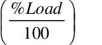 **= standard
rating part load ratio (PLR) points, 75%, 50%,
25%.
**= standard
rating part load ratio (PLR) points, 75%, 50%,
25%.
 =Full load heating
capacity (W) of the air-source heat pump equipment determined
from ANSI/AHRI Standard 550/590 and test conditions shown in
Table 49 for 100% load.
=Full load heating
capacity (W) of the air-source heat pump equipment determined
from ANSI/AHRI Standard 550/590 and test conditions shown in
Table 49 for 100% load.
 =Part load heating
capacity (W) of the air-source heat pump units determined from
ANSI/AHRI Standard 550/590 at the standard desired reduced
ambient test conditions as shown in Table 49 and the minimum
part load capacity of the unit.
=Part load heating
capacity (W) of the air-source heat pump units determined from
ANSI/AHRI Standard 550/590 at the standard desired reduced
ambient test conditions as shown in Table 49 and the minimum
part load capacity of the unit.
where,
 = Reference capacity
specified by the user, (W).
= Reference capacity
specified by the user, (W).
 = User-specified
bi-quadratic curve evaluated at full load (100%) test
conditions shown in Table 49, (dimensionless).
= User-specified
bi-quadratic curve evaluated at full load (100%) test
conditions shown in Table 49, (dimensionless).
 = Part load capacity (W)
of the chiller determined from ANSI/AHRI Standard 550/590 at
the standard desired reduced ambient test conditions as shown
in Table 49.
= Part load capacity (W)
of the chiller determined from ANSI/AHRI Standard 550/590 at
the standard desired reduced ambient test conditions as shown
in Table 49.
 = Minimum PLR up to which
chiller can be unloaded
= Minimum PLR up to which
chiller can be unloaded
| Standard Rating (Integrated Part
Load Value)<> |
Evaporator (All types)
1Condenser (Water Cooled)
1Condenser (Air Cooled)
1Condenser (Evaporatively Cooled)
Air-Cooled Without
Water and Evaporatively-
1 If the unit Manufacturer’s recommended minimum
temperatures are greater than those specified in Table 3, then
those may be used in lieu of the specified temperatures.
———————————————————————–
: Standard Rating (Integrated Part Load Value)
Electric
Chiller Model Based on Condenser Leaving Temperature[LINK]
This model (object name Chiller:Electric:ReformulatedEIR)
simulates the thermal performance of an electric liquid
chiller and the power consumption of its compressor(s). The
model, developed by Hydeman et al. (2002) as part of the
CoolTools™ project sponsored by Pacific Gas and Electric
Company (PG&E), is an empirical model similar to
EnergyPlus’ Chiller:Electric:EIR
model. The model uses performance information at reference
conditions along with three curve fits for cooling capacity
and efficiency to determine chiller operation at off-reference
conditions. The model has the same capabilities as the Chiller:Electric:EIR
model, but can potentially provide significant accuracy
improvement over the Chiller:Electric:EIR
model for chillers with variable-speed compressor motor drives
and/or variable condenser water flow applications.
Chiller performance curves can be generated by fitting
manufacturer’s catalog data or measured data. Performance
curves developed primarily from manufacturer’s performance
data are provided in the EnergyPlus Reference DataSets
(Chillers.idf and AllDataSets.idf). This chiller model can be
used to predict the performance of various chiller types
(e.g., reciprocating, screw, scroll, and centrifugal) with
water-cooled condensers. The model does not simulate the
thermal performance or the power consumption of associated
pumps or cooling towers. This auxiliary equipment must be
modeled using other EnergyPlus models
(e.g. CoolingTower:SingleSpeed).
The main difference between this model and the Chiller:Electric:EIR
model is the condenser fluid temperature used in the
associated performance curves: the Chiller:Electric:ReformulatedEIR
model uses the LEAVING condenser water temperature while the
Chiller:Electric:EIR
model uses the ENTERING condenser water temperature. In
addition, the Energy Input to Cooling Output Function of Part
Load Ratio curve for this reformulated EIR chiller model
includes the condenser leaving water temperature as an
independent variable in addition to part-load ratio. Since the
leaving condenser water temperature is a function of load,
chiller performance, and condenser entering water temperature,
EnergyPlus must iterate to converge on a solution for each
simulation time step.
Model Description[LINK]
The chiller model uses user-supplied performance
information at reference conditions along with three
performance curves (curve objects) for cooling capacity and
efficiency to determine chiller operation at off-reference
conditions. The three performance curves are:
- Cooling Capacity Function of Temperature Curve
- Energy Input to Cooling Output Ratio Function of
Temperature Curve
- Energy Input to Cooling Output Ratio Function of Part Load
Ratio Curve
The cooling capacity function of temperature curve is a
biquadratic performance curve with two independent variables:
the leaving chilled water temperature and the leaving
condenser water temperature. The output of this curve is
multiplied by the reference capacity to give the full-load
cooling capacity at specific temperature operating conditions
(i.e., at temperatures different from the reference
temperatures). The curve should have a value of 1.0 at the
reference temperatures and flow rates specified in the input
data file by the user. The biquadratic curve should be valid
for the range of water temperatures anticipated for the
simulation (otherwise the program issues warning
messages).
where
ChillerCapFTemp = Cooling capacity factor, equal
to 1 at reference conditions
Tcw,l= leaving chilled water
temperature, ˚C
Tcond,l= leaving condenser water
temperature, ˚C. This will be the water temperature entering
the condenser loop (e.g., entering the cooling tower). If the
chiller is a heat recovery chiller,then the condenser leaving
temperature is adjusted to account for both fluid streams as
described in the section above on heat recovery chillers.
- The energy input to cooling output ratio function of
temperature curve is a biquadratic performance curve that
parameterizes the variation of the energy input to cooling
output ratio (EIR) as a function of the leaving chilled water
temperature and the leaving condenser water temperature. The
EIR is the inverse of the COP. The output of this curve is
multiplied by the reference EIR (inverse of the reference COP)
to give the full-load EIR at specific temperature operating
conditions (i.e., at temperatures different from the reference
temperatures). The curve should have a value of 1.0 at the
reference temperatures and flow rates specified in the input
data file by the user. The biquadratic curve should be valid
for the range of water temperatures anticipated for the
simulation (otherwise the program issues warning
messages).
 where
where
ChillerEIRFTemp = Energy input to cooling output
factor, equal to 1 at reference conditions
Tcw,l = leaving chilled water
temperature, ˚C
Tcond,l= leaving condenser water
temperature, ˚C. This will be the water temperature entering
the condenser loop (e.g., entering the cooling tower). If the
chiller is a heat recovery chiller,then the condenser leaving
temperature is adjusted to account for both fluid streams as
described in the section above on heat recovery chillers.
- The energy input to cooling output ratio function of
part-load ratio curve is a bicubic performance curve that
parameterizes the variation of the chiller input power ratio
as a function of the leaving condenser water temperature and
the part-load ratio. The part-load ratio is the actual cooling
load divided by the chiller’s available cooling capacity. The
output of this curve is multiplied by the reference EIR
(inverse of the reference COP) and the Energy Input to Cooling
Output Ratio Function of Temperature Curve to give the EIR at
the specific temperatures and part-load ratio at which the
chiller is operating. This curve should have a value of 1.0 at
the reference leaving condenser water temperature with
part-load ratio equal to 1.0. It is recommended that this
performance curve be developed using both full- and part-load
performance data. The bicubic curve should be valid for the
range of condenser water temperatures and part-load ratios
anticipated for the simulation (otherwise the program issues
warning messages).
where
ChillerEIRFPLR = Energy input to cooling output
factor, equal to 1 at the reference leaving condenser water
temperature and PLR = 1.0
Tcond,l= leaving condenser water
temperature, ˚C. This will be the water temperature entering
the condenser loop (e.g., entering the cooling tower). If the
chiller is a heat recovery chiller,then the condenser leaving
temperature is adjusted to account for both fluid streams as
described in the section above on heat recovery chillers.
PLR = Part load ratio = (cooling load) /
(chiller’s available cooling capacity)
Pchiller = chiller power at specific
PLR
Pref =
/COPref
Note: Although a bicubic curve requires 10 coefficients
(ref. Curve:Bicubic), coefficients 7, 9 and 10 are typically
not used in the performance curve described here and should be
entered as 0 unless sufficient performance data and regression
accuracy exist to justify the use of these terms of the
bicubic curve.
All three of the performance curves are accessed through
EnergyPlus’ built-in performance curve equation manager
(curve:biquadratic and curve:bicubic). Note that the above
three performance curves use the leaving condenser water
temperature as an independent variable, instead of the
entering condenser water temperature used in the performance
curves for the Chiller:Electric:EIR
model. Since the leaving condenser water temperature is
calculated based on the condenser heat transfer rate, which is
a function of the load to be met by the chiller, chiller
compressor power, and the false loading (detailed calculations
are given below), iterative calculations are required to
determine the actual (converged) leaving condenser water
temperature. The program uses the leaving condenser water
temperature from the previous iteration to calculate values
for each of the three performance curves described above.
After obtaining the condenser heat transfer rate, the leaving
condenser water temperature is recalculated. When the
difference between the leaving condenser water temperature
calculated on successive iterations is less than
0.0001°C, the solution is assumed to have
converged. Warning messages are issued if the calculated
solution for leaving condenser water temperature and/or
part-load ratio falls outside the valid range specified for
the chiller’s performance curves. If these warnings are
issued, the user may chose to extend the range for the
performance curves (only if a small extension is required
since model extrapolation may produce significant errors) or a
different chiller and associated performance curves with
extended performance range can be located and used for the
simulation.
Note: Chiller:Electric:ReformulatedEIR
objects and their associated performance curve objects are
developed using performance information for a specific chiller
and should almost always be used together for an EnergyPlus
simulation. Changing the object input values, or swapping
performance curves between chillers, should be done with
extreme caution. For example, if the user wishes to model a
chiller size that is different from the reference capacity, it
is highly recommended that the reference flow rates be scaled
proportionately to the change in reference capacity. Although
this model can provide more accurate prediction than the Chiller:Electric:EIR
model, it requires more performance data to develop the
associated performance curves (at least 12 points from
full-load performance and 7 points from part-load
performance).
Although performance curve data sets for 160 chillers are
provided in the EnergyPlus Reference DataSets (Chillers.idf
and AllDataSets.idf), they may not meet the requirements for
specific applications. One can develop performance curves from
performance data using two available techniques (Hydeman and
Gillespie 2002). The first technique is called the
Least-squares Linear Regression method and is used when
sufficient performance data exist to employ standard
least-square linear regression techniques. The second
technique is called Reference Curve Method and is used when
insufficient performance data exist to apply linear regression
techniques. A detailed description of both techniques can be
found in the reference mentioned above.
For any simulation time step, the chiller’s available
cooling capacity is calculated as follows:
where
 = chiller capacity at
reference conditions (reference temperatures and flow rates
defined by the user), W
= chiller capacity at
reference conditions (reference temperatures and flow rates
defined by the user), W
 = available chiller
capacity adjusted for current water temperatures, W
= available chiller
capacity adjusted for current water temperatures, W
The model then calculates the evaporator heat transfer rate
required to bring the entering chilled water temperature down
to the leaving chilled water setpoint temperature (established
using a SetpointManager object and referenced in the PlantLoop
object). If this calculated heat transfer rate is greater than
the heat transfer rate being requested by the plant equipment
operation scheme, then the evaporator heat transfer rate is
reset to the requested cooling rate.
The evaporator heat transfer rate is then compared to the
available capacity. If the available chiller capacity is
sufficient to meet the evaporator heat transfer rate, the
leaving chilled water temperature is set equal to the chilled
water setpoint temperature. If the requested evaporator heat
transfer rate is larger than the available capacity the
chilled water leaving the evaporator is allowed to float
upward. For this case, the exiting chilled water temperature
is calculated based on the water temperature entering the
evaporator, the available cooling capacity, and the evaporator
mass flow rate as follows:
where
Tcw,l= water temperature leaving the
evaporator, ˚C
Tcw,e= water temperature entering the
evaporator, ˚C
= evaporator mass flow
rate, kg/s
Cp,evap= specific heat of water
entering evaporator at Tcw,e, J/kg-˚C
The part-load ratio is then calculated as the ratio of the
evaporator heat transfer rate to the available chiller
capacity. The part-load ratio is not allowed to be greater
than the maximum part-load ratio specified by the user or less
than zero as follows:
where
PLR= part-load ratio
= load to be met by the
chiller, W
PLRmax= maximum part-load ratio (specified
by the user in the input data file)
Note that the maximum part-load ratio (PLRmax,
specified in the Chiller:Electric:ReformulatedEIR
object) used in the equation should be less than or equal to
the maximum part-load ratio specified in the “Energy Input to
Cooling Output Ratio Function of Part-Load Ratio” performance
curve object.
The model assumes that the cooling load is met through
chiller unloading down to the minimum unloading ratio. False
loading (e.g. hot-gas bypass) is assumed to occur between the
minimum unloading ratio and the minimum part-load ratio
yielding constant electrical power consumption under these
conditions. Below the minimum part-load ratio, the chiller
cycles on/off to meet very small loads and the power
consumption during the on cycle is the same as when the
chiller is operating at the minimum part load ratio. When the
chiller part-load ratio is less than the minimum part-load
ratio, the on-off cycling ratio of the chiller is calculated
as follows and is available as an output variable.
To properly account for chiller electric power consumption
when PLR is less than the minimum unloading ratio, the PLR is
reset to the greater of the PLR calculated above and the PLR
at the minimum unloading ratio. The result is available as the
output variable Chiller Part Load Ratio.
This revised PLR accounts for the “false loading” (e.g.,
hot-gas bypass) that is assumed to occur whenever the PLR
(based on cooling load divided by available capacity) is less
than the minimum unloading ratio specified. The amount of
false loading on the chiller is calculated using this revised
PLR and is reported as an output variable as follows:
The electrical power consumption for the chiller
compressor(s) for any simulation time step is then calculated
using the following equation:
 where
where
Pchiller= Chiller compressor power,
W
COPref= Reference coefficient of
performance, W/W
Heat rejected by the chiller condenser includes the heat
transferred in the evaporator plus a portion or all of the
compressor electrical energy consumption. For electric
chillers with hermetic compressors, all compressor energy
consumption is rejected by the condenser (compressor motor
efficiency = effmotor = 1.0). For chillers
with semi-hermetic or open compressors, only a portion of the
compressor energy use is rejected by the condenser. The heat
transfer rate for the chiller condenser is calculated as
follows:
where
= condenser heat transfer
rate, W
= compressor motor
efficiency = fraction of compressor electrical energy
consumption rejected as condenser heat
The above curve values are calculated based on the leaving
condenser water temperature found through iteration. After
obtaining the condenser heat transfer rate, the final leaving
condenser water temperature is then calculated as:
where:
Tcond,l= water temperature leaving the
condenser, ˚C
Tcond,e= water temperature entering the
condenser, ˚C
= mass flow rate through
the condenser, kg/s
= specific heat of water
entering the condenser at Tcond,e,
J/kg-˚C
The final calculations determine the total heat transfer
energy for the condenser and evaporator, as well as the total
electric energy consumed by the chiller compressor motor(s)
and condenser fan(s). The results are available as output
variables.
where
Qcond= chiller condenser heat transfer
energy, J
Qevap= chiller evaporator cooling
energy, J
Echiller= chiller (compressor) electric
energy, J
Econd= chiller condenser fan electric
energy, J
TimeStepSys = HVAC system simulation time step,
hr
= conversion factor,
sec/hr
Heat from the electric reformulated EIR chiller condenser
may be recovered. The heat recovery water flow rate is
specified by the user along with the input and output nodes
connected to the heat recovery loop. The algorithms are
identical to those used for Chiller:Electric
and Chiller:Electric:EIR.
Refer to the section entitled Chillers with Plant Heat
Recovery for details.
Standard
Rating (Integrated Part Load Value)[LINK]
Integrated Part Laod Value (IPLV) calculations for
Reformulated EIR chiller are similar to what are described
above for EIR chillers. The only difference with Reformulated
EIR chiller is that it calls an iterative subroutine
(SolveRegulaFalsi) to obtain a condenser water outlet
temperature which corresponds to condenser inlet temperature
at reduced capacity conditions as outlined in Table 49 above.
SolveRegulaFalsi is a general utility routine for finding the
zero of a function. In this case it finds the condenser inlet
temperature that will zero the residual function – the
difference between calculated condenser inlet temperature and
desired condenser inlet temperature per ANSI/AHRE 550/590,
2011 (table 42 above) divided by desired condenser inlet
temperature.
Hydeman, M., N. Webb, P. Sreedharan, and S. Blanc. 2002.
Development and Testing of a Reformulated Regression-Based
Electric Chiller Model. ASHRAE Transactions HI-02-18-2.
Hydeman, M. and K.L. Gillespie. 2002. Tools and Techniques
to Calibrate Electric Chiller Component Models. ASHRAE
Transactions AC-02-9-1.
Hydeman, M., K. Gillespie, and R. Kammerud. 1997.
PG&E’s CoolTools project: A toolkit to improve evaluation
and operation of chilled water plants. Presented at the
Cool$ense National Forum on Integrated Chilled Water
Retrofits, Sep. 1997. Berkeley California: Lawrence Berkeley
National Laboratory.
Engine Driven Chiller[LINK]
The engine driven chiller (Object name:
Chiller:EngineDriven) is the empirical model from the Building
Loads and System Thermodynamics (BLAST) program. Fitting
catalog data to a third order polynomial equations generates
the chiller performance curves. Three sets of coefficients are
required to model the open centrifugal chiller as discussed in
the section, titled, ‘Electric Chiller Based on BLAST
Centrifugal Chiller Model’. Additional curve fits are required
to model the engine. Because the model inherently involves the
lower heating value of the fuel, a reference temperature is
also involved in the calculations, which manufacturers present
at 25°C.
The engine model was also developed for the BLAST program.
It was adapted for use in EnergyPlus. This model is used for
both the engine driven generator and the engine driven
chiller. It uses the following set of equations all of which
are quadratic fits to the PLR (Part Load Ratio) of the
generator. The coefficients must be derived from manufacturers
data.
The exhaust gas temp and flow rate are used if a stack heat
exchanger is used to recover waste heat from the exhaust. This
temperature is the inlet temperature to the heat exchanger
which is modeled in a UA-effectiveness form:
The exhaust flow rate is then calculated as:
where Treference is the reference temperature
for the fuel lower heating value, and is given as 25°C in
manufacturer’s data, and
Finally, heat recovered from the lube oil and the water
jacket are accounted for as follows:
Chiller Basin Heater[LINK]
Calculations are also made to estimate the electric power
input to the basin heater for chillers with
evaporatively-cooled condensers. The chillers which calculate
basin heater power are Chiller:Electric:EIR,
Chiller:Electric,
Chiller:ConstantCOP,
Chiller:EngineDriven
and Chiller:CombustionTurbine.
A schedule may be used to disable the basin heater during
regular maintenance periods or other time periods (e.g.,
during summer). If a schedule is not provided, the basin
heater is assumed to be available the entire simulation time
period. The basin heater operates when it is scheduled on, the
outdoor air dry-bulb temperature is below the basin heater
setpoint temperature, and the chiller is not active (i.e.,
chiller is not operating for the simulation time step — for
example, when there is no cooling load to be met by the
chiller, or if there is no water flow through the chiller
due to a chiller or pump availability schedule, etc.).
The user is required to enter a basin heater capacity (watts
per degree Kelvin) and a heater setpoint temperature
(oC) if they want to model basin heater electric
power.
where:
 = Chiller basin heater
electric power (W)
= Chiller basin heater
electric power (W)
 = Chiller basin heater
electric consumption (J)
= Chiller basin heater
electric consumption (J)
Tsetpoint,basin = Basin heater setpoint
temperature, user input (oC)
Tdb,outdoor = Outdoor air dry-bulb
temperature (oC)
CAPheater,basin = Basin heater
capacity, user input (W/K)
Scheduleheater,basin = Basin heater
schedule, user input (schedule value > 0 means ON)
ChillerIsOFF = Logical variable denoting that the
chiller is not operating for the current simulation time step
(e.g., there is no cooling load to be met by the chiller, or
if there is no water flow through the chiller due to a chiller
or pump availability schedule, etc.)

Chillers[LINK]
Absorption Chiller[LINK]
The input object Chiller:Absorption provides a model for absorption chillers that is an empirical model of a standard absorption refrigeration cycle. The condenser and evaporator are similar to that of a standard chiller, which are both water-to-water heat exchangers. The assembly of a generator and absorber provides the compression operation. Low-pressure vapor from the evaporator is absorbed by the liquid solution in the absorber. A pump receives low-pressure liquid from the absorber, elevates the pressure of the liquid, and delivers the liquid to the generator. In the generator, heat from a high temperature source (hot water or steam) drives off the vapor that has been absorbed by the solution. The liquid solution returns to the absorber through a throttling valve whose purpose is to provide a pressure drop to maintain the pressure difference between the generator and absorber. The heat supplied to the absorber can be waste heat from a diesel jacket, or the exhaust heat from diesel, gas, and steam turbines. For more information on absorption chillers, see the Input/Output Reference Document (Object: Chiller:Absorption).
The part-load ratio of the absoprtion chiller’s evaporator is simply the actual cooling effect produced by the chiller divided by the maximum cooling effect available.
where
This absorption chiller model is based on a polynomial fit of absorber performance data. The Generator Heat Input Part Load Ratio Curve is a quadratic equation that determines the ratio of the generator heat input to the demand on the chiller’s evaporator (Qevap).
The Pump Electric Use Part Load Ratio Curve is a quadratic equation that determines the ratio of the actual absorber pumping power to the nominal pumping power.
Thus, the coefficient sets establish the ratio of heat power in-to-cooling effect produced as a function of part load ratio. The ratio of heat-power-in to cooling-effect-produced is the inverse of the coefficient of performance.
If the operating part-load ratio is greater than the minimum part-load ratio, the chiller will run the entire time step and cycling will not occur (i.e. CyclingFrac = 1). If the operating part-load ratio is less than the minimum part-load ratio, the chiller will be on for a fraction of the time step equal to CyclingFrac. Steam (or hot water) and pump electrical energy use are also calculated using the chiller part-load cycling fraction.
where
The evaporator water mass flow rate is calculated based on the Chiller Flow Mode as follows.
Constant Flow Chillers:
Variable Flow Chillers:
where
The evaporator outlet water temperature is then calculated based on the cooling effect produced and the evaporator entering water temperature.
where
The condenser heat transfer and condenser leaving water temperature are also calculated.
where
The absorption chiller can model the impact of steam or hot water entering the generator, although the connection of the steam (hot water) nodes to a plant is not actually required. The calculations specific to the generator depend on the type of fluid used and are described here in further detail.
Steam Loop Calculations[LINK]
When a steam loop is used and the inlet and outlet node names are specified (i.e. the nodes are connected to a steam loop), the generator outlet node steam mass flow rate and temperature are calculated based on the generator input power, latent heat of steam, the specific heat of water, and the amount of subcooling in the steam generator. The model assumes dry saturated steam enters the absorption chiller’s generator and exits the generator as a subcooled liquid. The temperature leaving the generator is calculated based on the user entered amount of liquid subcooling in the generator. The effect of subcooling of the liquid (condensate) in the pipe returning to the boiler is not modeled.
where
Hot Water Loop Calculations[LINK]
When a hot water loop is used and the inlet and outlet node names are specified (i.e. the nodes are connected to a hot water loop), the generator outlet node temperature is calculated based on the generator input power, mass flow rate of water, and the specific heat of water entering the hot water generator. The calculations are based on the Chiller Flow Mode as follows.
Constant Flow Chillers:
Variable Flow Chillers:
where
Indirect Absorption Chiller[LINK]
The Chiller:Absorption:Indirect object is an enhanced version of the absorption chiller model found in the Building Loads and System Thermodynamics (BLAST) program. This enhanced model is nearly identical to the existing absorption chiller model (Ref. Chiller:Absorption) with the exceptions that: 1) the enhanced indirect absorption chiller model provides more flexible performance curves and 2) chiller performance now includes the impact of varying evaporator, condenser, and generator temperatures. Since these absorption chiller models are nearly identical (i.e., the performance curves of the enhanced model can be manipulated to produce similar results to the previous model), it is quite probable that the Chiller:Absorption model will be deprecated in a future release of EnergyPlus.
The indirect absorption chiller’s condenser and evaporator are similar to that of a standard chiller, which are both water-to-water heat exchangers. The assembly of a generator and absorber provides the compression operation. A schematic of a single-stage absorption chiller is shown in the figure below. Low-pressure vapor from the evaporator is absorbed by the liquid solution in the absorber. A pump receives low-pressure liquid from the absorber, elevates the pressure of the liquid, and delivers the liquid to the generator. In the generator, heat from a high temperature source (hot water or steam) drives off the vapor that has been absorbed by the solution. The liquid solution returns to the absorber through a throttling valve whose purpose is to provide a pressure drop to maintain the pressure difference between the generator and absorber. The heat supplied to the generator can be either hot water or steam, however, connection to an actual plant loop is not required. For more information on indirect absorption chillers, see the Input/Output Reference Document (Object: Chiller:Absorption:Indirect).
The chiller cooling effect (capacity) will change with a change in condenser water temperature. Similarly, the chiller cooling effect will change as the temperature of the evaporator water changes. The chiller cooling effect will also change with a change in or generator inlet water temperature and only applies when Hot Water is used as the generator heat source. A quadratic or cubic equation is used to modify the rated chiller capacity as a function of both the condenser and generator inlet water temperatures and the evaporator outlet water temperature. If any or all of the capacity correction factor curves are not used, the correction factors are assumed to be 1.
where
The part-load ratio of the indirect absoprtion chiller’s evaporator is simply the actual cooling effect required (load) divided by the maximum cooling effect available.
where
The generator’s heat input is also a function of several parameters. The primary input for determining the heat input requirements is the Generator Heat Input function of Part-Load Ratio Curve. The curve is a quadratic or cubic equation that determines the ratio of the generator heat input to the chiller’s maximum capacity (Q~evap, max~) and is soley a function of part-load ratio. Typical generator heat input ratios at full load (i.e., PLR=1) are between 1 and 2. Two additional curves are available to modifiy the heat input requirement based on the generator inlet water temperature and the evaporator outlet water temperature.
where
GeneratorHIR = ratio of generator heat input to chiller operating capacity
GenfCondT = heat input modifier based on generator inlet water temperature
GenfEvapT = heat input modifier based on evaporator outlet water temperature
The Pump Electric Use function of Part-Load Ratio Curve is a quadratic or cubic equation that determines the ratio of the actual absorber pumping power to the nominal pumping power.
If the chiller operating part-load ratio is greater than the minimum part-load ratio, the chiller will run the entire time step and cycling will not occur (i.e. CyclingFrac = 1). If the operating part-load ratio is less than the minimum part-load ratio, the chiller will be on for a fraction of the time step equal to CyclingFrac. Generator heat input and pump electrical energy use are also calculated using the chiller part-load cycling fraction.
where
The evaporator water mass flow rate is calculated based on the Chiller Flow Mode as follows.
Constant Flow Chillers:
Variable Flow Chillers:
where
The evaporator outlet water temperature is then calculated based on the cooling effect produced and the evaporator entering water temperature.
where
The condenser heat transfer and condenser leaving water temperature are also calculated.
where
The absorption chiller can model the impact of steam or hot water entering the generator, although the connection of the steam (hot water) nodes to a plant is not actually required. The calculations specific to the generator depend on the type of fluid used and are described here in further detail.
Steam Loop Calculations[LINK]
When a steam loop is used and the inlet and outlet node names are specified (i.e. the nodes are connected to a steam loop), the generator outlet node steam mass flow rate and temperature are calculated based on the generator heat input, latent heat of steam, the specific heat of water, and the amount of subcooling in the steam generator. The model assumes dry saturated steam enters the generator and exits the generator as a subcooled liquid. The temperature leaving the generator is calculated based on the user entered amount of liquid subcooling in the generator. The effect of subcooling of the liquid (condensate) in the pipe returning to the boiler is also modeled using the user entered abount of steam condensate loop subcooling.
where
Hot Water Loop Calculations[LINK]
When a hot water loop is used and the inlet and outlet node names are specified (i.e. the nodes are connected to a hot water loop), the generator outlet node temperature is calculated based on the generator heat input, mass flow rate of water, and the specific heat of water entering the hot water generator. The calculations are based on the Chiller Flow Mode as follows.
Constant Flow Chillers:
Variable Flow Chillers:
where
Combustion Turbine Chiller[LINK]
The input object Chiller:CombustionTurbine provides a chiller model that is the empirical model from the Building Loads and System Thermodynamics (BLAST) program. Fitting catalog data to a third order polynomial equations generates the chiller performance curves. Three sets of coefficients are required to model the open centrifugal chiller as discussed in the section, titled, ‘Electric Chiller Based on BLAST Centrifugal Chiller Model’.
The gas turbine-driven chiller is an open centrifugal chiller driven directly by a gas turbine. The BLAST model of an open centrifugal chiller is modeled as standard vapor compression refrigeration cycle with a centrifugal compressor driven by a shaft power from an engine. The centrifugal compressor has the incoming fluid entering at the eye of a spinning impeller that throws the fluid by centrifugal force to the periphery of the impeller. After leaving the compressor, the refrigerant is condensed to liquid in a refrigerant to water condenser. The heat from the condenser is rejected to a cooling tower, evaporative condenser, or well water condenser depending on which one is selected by the user based on the physical parameters of the plant. The refrigerant pressure is then dropped through a throttling valve so that fluid can evaporate at a low pressure that provides cooling to the evaporator. The evaporator can chill water that is pumped to chilled water coils in the building. For more information, see the Input/Output Reference Document.
This chiller is modeled like the electric chiller with the same numerical curve fits and then some additional curve fits to model the turbine drive. Shown below are the definitions of the curves that describe this model.
The chiller’s temperature rise coefficient which is defined as the ratio of the required change in condenser water temperature to a given change in chilled water temperature, which maintains the capacity at the nominal value. This is calculated as the following ratio:
Where:
TCEntrequired = Required entering condenser air or water temperature to maintain rated capacity.
TCEntrated = Rated entering condenser air or water temperature at rated capacity.
TELvrequired = Required leaving evaporator water outlet temperature to maintain rated capacity.
TELvrated = Rated leaving evaporator water outlet temperature at rated capacity.
The Capacity Ratio Curve is a quadratic equation that determines the Ratio of Available Capacity to Nominal Capacity. The defining equation is:
Where the Delta Temperature is defined as:
TempCondIn = Temperature entering the condenser (water or air temperature depending on condenser type).
TempCondInDesign = Temp Design Condenser Inlet from User input above.
TempEvapOut = Temperature leaving the evaporator.
TempEvapOutDesign = Temp Design Evaporator Outlet from User input above.
TempRiseCoefficient = User Input from above.
The following three fields contain the coefficients for the quadratic equation.
The Power Ratio Curve is a quadratic equation that determines the Ratio of Full Load to Power. The defining equation is:
The Full Load Ratio Curve is a quadratic equation that determines the fraction of full load power. The defining equation is:
The Fuel Input Curve is a polynomial equation that determines the Ratio of Fuel Input to Energy Output. The equation combines both the Fuel Input Curve Coefficients and the Temperature Based Fuel Input Curve Coefficients. The defining equation is:
Where FIC represents the Fuel Input Curve Coefficients, TBFIC represents the Temperature Based Fuel Input Curve Coefficients, Rload is the Ratio of Load to Combustion Turbine Engine Capacity, and ATairis the difference between the current ambient and design ambient temperatures.
The Exhaust Flow Curve is a quadratic equation that determines the Ratio of Exhaust Gas Flow Rate to Engine Capacity. The defining equation is:
Where GTCapacity is the Combustion Turbine Engine Capacity, and ATair is the difference between the current ambient and design ambient temperatures.
The Exhaust Gas Temperature Curve is a polynomial equation that determines the Exhaust Gas Temperature. The equation combines both the Exhaust Gas Temperature Curve Coefficients (Based on the Part Load Ratio) and the (Ambient) Temperature Based Exhaust Gas Temperature Curve Coefficients. The defining equation is:
Where C represents the Exhaust Gas Temperature Curve Coefficients, TBC are the Temperature Based Exhaust Gas Temperature Curve Coefficients, RLoad is the Ratio of Load to Combustion Turbine Engine Capacity, and ATair is the difference between the actual ambient and design ambient temperatures.
The Recovery Lubricant Heat Curve is a quadratic equation that determines the recovery lube energy. The defining equation is:
Where Pload is the engine load and RL is the Ratio of Load to Combustion Turbine Engine Capacity
The UA is an equation that determines the overall heat transfer coefficient for the exhaust gasses with the stack. The heat transfer coefficient ultimately helps determine the exhaust stack temperature. The defining equation is:
Chiller Basin Heater[LINK]
This chiller’s basin heater (for evaporatively-cooled condenser type) operates in the same manner as the Engine driven chiller’s basin heater. The calculations for the chiller basin heater are described in detail at the end of the engine driven chiller description (Ref. Engine Driven Chiller).
ChillerHeater:Absorption:DirectFired[LINK]
Overview[LINK]
This model (object name ChillerHeater:Absorption:DirectFired) simulates the performance of a direct fired two-stage absorption chiller with optional heating capability. The model is based on the direct fired absorption chiller model (ABSORG-CHLR) in the DOE-2.1 building energy simulation program. The EnergyPlus model contains all of the features of the DOE-2.1 chiller model, plus some additional capabilities.
This model simulates the thermal performance of the chiller and the fuel consumption of the burner(s). This model does not simulate the thermal performance or the power consumption of associated pumps or cooling towers. This auxiliary equipment must be modeled using other EnergyPlus models (e.g. Cooling Tower:Single Speed).
Model Description[LINK]
The chiller model uses user-supplied performance information at design conditions along with five performance curves (curve objects) for cooling capacity and efficiency to determine chiller operation at off-design conditions. Two additional performance curves for heating capacity and efficiency are used when the chiller is operating in a heating only mode or simultaneous cooling and heating mode.
Cooling[LINK]
The following nomenclature is used in the cooling equations:
AvailCoolCap=available full-load cooling capacity at current conditions [W]
CEIR=user input “Electric Input to Cooling Output Ratio”
CEIRfPLR=electric input to cooling output factor, equal to 1 at full load, user input “Electric Input to Cooling Output Ratio Function of Part Load Ratio Curve Name”
CEIRfT=electric input to cooling output factor, equal to 1 at design conditions, user input “Electric Input to Cooling Output Ratio Function of Temperature Curve Name”
CFIR=user input “Fuel Input to Cooling Output Ratio”
CFIRfPLR=fuel input to cooling output factor, equal to 1 at full load, user input “Fuel Input to Cooling Output Ratio Function of Part Load Ratio Curve Name”
CFIRfT=fuel input to cooling output factor, equal to 1 at design conditions, user input “Fuel Input to Cooling Output Ratio Function of Temperature Curve Name”
CondenserLoad=condenser heat rejection load [W]
CoolCapfT=cooling capacity factor, equal to 1 at design conditions, user input “Cooling Capacity Function of Temperature Curve Name”
CoolElectricPower=cooling electricity input [W]
CoolFuelInput=cooling fuel input [W]
CoolingLoad=current cooling load on the chiller [W]
CPLR=cooling part-load ratio = CoolingLoad / AvailCoolCap
HeatingLoad=current heating load on the chiller heater [W]
HFIR=user input “Fuel Input to Heating Output Ratio”
HPLR=heating part-load ratio = HeatingLoad / AvailHeatCap
MinPLR=user input “Minimum Part Load Ratio”
NomCoolCap=user input “Nominal Cooling Capacity” [W]
RunFrac=fraction of time step which the chiller is running
Tcond=entering or leaving condenser fluid temperature [C]. For a water-cooled condenser this will be the water temperature returning from the condenser loop (e.g., leaving the cooling tower) if the entering condenser fluid temperature option is used. For air- or evap-cooled condensers this will be the entering outdoor air dry-bulb or wet-bulb temperature, respectively, if the entering condenser fluid temperature option is used.
Tcw,l=leaving chilled water temperature [C]
Five performance curves are used in the calculation of cooling capacity and efficiency:
The cooling capacity function of temperature (CoolCapfT) curve represents the fraction of the cooling capacity of the chiller as it varies by temperature. This a biquadratic curve with the input variables being the leaving chilled water temperature and either the entering or leaving condenser fluid temperature. The output of this curve is multiplied by the nominal cooling capacity to give the full-load cooling capacity at specific temperature operating conditions (i.e., at temperatures different from the design temperatures). The curve should have a value of 1.0 at the design temperatures and flow rates specified in the input data file by the user. The biquadratic curve should be valid for the range of water temperatures anticipated for the simulation.
The available cooling capacity of the chiller is then computed as follows:
The fuel input to cooling output ratio function of temperature (CFIRfT) curve represents the fraction of the fuel input to the chiller at full load as it varies by temperature. This a biquadratic curve with the input variables being the leaving chilled water temperature and either the entering or leaving condenser fluid temperature. The output of this curve is multiplied by the nominal fuel input to cooling output ratio (CFIR) to give the full-load fuel input to cooling capacity ratio at specific temperature operating conditions (i.e., at temperatures different from the design temperatures). The curve should have a value of 1.0 at the design temperatures and flow rates specified in the input data file by the user. The biquadratic curve should be valid for the range of water temperatures anticipated for the simulation.
The fuel input to cooling output ratio function of part load ratio (CFIRfPLR) curve represents the fraction of the fuel input to the chiller as the load on the chiller varies at a given set of operating temperatures. The curve is normalized so that at full load the value of the curve should be 1.0. The curve is usually linear or quadratic.
The fraction of the time step during which the chiller heater is operating is computed as a function of the cooling and heating part-load ratios and the user-input minimum part-load ratio:
The cooling fuel input to the chiller is then computed as follows:
The electric input to cooling output ratio as function of temperature (CEIRfT) curve represents the fraction of electricity to the chiller at full load as it varies by temperature. This a biquadratic curve with the input variables being the leaving chilled water temperature and either the entering or leaving condenser fluid temperature.
The electric input to cooling output ratio function of part load ratio (CEIRfPLR) curve represents the fraction of electricity to the chiller as the load on the chiller varies at a given set of operating temperatures. The curve is normalized so that at full load the value of the curve should be 1.0. The curve is usually linear or quadratic.
The cooling electric input to the chiller is computed as follows:
All five of these cooling performance curves are accessed through EnergyPlus’ built-in performance curve equation manager (objects Curve:Linear, Curve:Quadratic and Curve:Biquadratic). It is not imperative that the user utilize all coefficients in the performance curve equations if their performance equation has fewer terms (e.g., if the user’s CFIRfPLR performance curve is linear instead of quadratic, simply enter the values for a and b, and set coefficient c equal to zero).
The condenser load is computed as follows:
Heating[LINK]
The following nomenclature is used in the heating equations:
AvailHeatCap=available full-load heating capacity at current conditions [W]
CPLRh=cooling part-load ratio for heating curve = CoolingLoad / NomCoolCap
HeatCapfCPLR=heating capacity factor as a function of cooling part load ratio, equal to 1 at zero cooling load, user input “Heating Capacity Function of Cooling Capacity Curve Name”
HeatCoolCapRatio=user input “Heating to Cooling Capacity Ratio”
HeatElectricPower=heating electricity input [W]
HeatFuelInput=heating fuel input [W]
HeatingLoad=current heating load on the chiller [W]
HEIR=user input “Electric Input to Heating Output Ratio”
HFIR=user input “Fuel Input to Heating Output Ratio”
HFIRfHPLR=fuel input to heating output factor, equal to 1 at full load, user input “Fuel Input to Heat Output Ratio During Heating Only Operation Curve Name”
HPLR=heating part-load ratio = HeatingLoad / AvailHeatCap
MinPLR=user input “Minimum Part Load Ratio”
NomCoolCap=user input “Nominal Cooling Capacity” [W]
RunFrac=fraction of time step which the chiller is running
TotalElectricPower=total electricity input [W]
TotalFuelInput=total fuel input [W]
Cooling is the primary purpose of the Direct Fired Absorption Chiller so that function is satisfied first and if energy is available for providing heating that is provided next.
The two performance curves for heating capacity and efficiency are:
The heating capacity function of cooling capacity curve (HeatCapfCool) determines how the heating capacity of the chiller varies with cooling capacity when the chiller is simultaneously heating and cooling. The curve is normalized so an input of 1.0 represents the nominal cooling capacity and an output of 1.0 represents the full heating capacity. An output of 1.0 should occur when the input is 0.0.
The available heating capacity is then computed as follows:
The fuel input to heat output ratio curve (HFIRfHPLR) function is used to represent the fraction of fuel used as the heating load varies as a function of heating part load ratio. It is normalized so that a value of 1.0 is the full available heating capacity. The curve is usually linear or quadratic and will probably be similar to a boiler curve for most chillers.
The fraction of the time step during which the chiller is operating is computed as a function of the cooling and heating part-load ratios and the user-input minimum part-load ratio:
The heating electric input to the chiller is computed as follows:
If the chiller is delivering heating and cooling simultaneously, the parasitic electric load will be double-counted, so the following logic is applied:
The total fuel and electric power input to the chiller is computed as shown below:
ChillerHeater:Absorption:DoubleEffect[LINK]
Overview[LINK]
This model (object name ChillerHeater:Absorption:DoubleEffect) simulates the performance of an exhaust fired two-stage (double effect) absorption chiller with optional heating capability. The model is based on the direct fired absorption chiller model (ABSORG-CHLR) in the DOE-2.1 building energy simulation program. The EnergyPlus model contains all of the features of the DOE-2.1 chiller model, plus some additional capabilities. The model uses the exhaust gas output from Microturbine.
This model simulates the thermal performance of the chiller and the thermal energy input to the chiller. This model does not simulate the thermal performance or the power consumption of associated pumps or cooling towers. This auxiliary equipment must be modeled using other EnergyPlus models (e.g. Cooling Tower:Single Speed).
Model Description[LINK]
The chiller model uses user-supplied performance information at design conditions along with five performance curves (curve objects) for cooling capacity and efficiency to determine chiller operation at off-design conditions. Two additional performance curves for heating capacity and efficiency are used when the chiller is operating in a heating only mode or simultaneous cooling and heating mode.
Cooling[LINK]
The following nomenclature is used in the cooling equations:
AvailCoolCap=available full-load cooling capacity at current conditions [W]
CEIR=user input “Electric Input to Cooling Output Ratio”
CEIRfPLR=electric input to cooling output factor, equal to 1 at full load, user input “Electric Input to Cooling Output Ratio Function of Part Load Ratio Curve Name”
CEIRfT=electric input to cooling output factor, equal to 1 at design conditions, user input “Electric Input to Cooling Output Ratio Function of Temperature Curve Name”
TeFIR=user input “Thermal Energy Input to Cooling Output Ratio”
TeFIRfPLR=thermal energy input to cooling output factor, equal to 1 at full load, user input “Thermal Energy Input to Cooling Output Ratio Function of Part Load Ratio Curve Name”
TeFIRfT=thermal energy input to cooling output factor, equal to 1 at design conditions, user input “Thermal Energy Input to Cooling Output Ratio Function of Temperature Curve Name”
CondenserLoad=condenser heat rejection load [W]
CoolCapfT=cooling capacity factor, equal to 1 at design conditions, user input “Cooling Capacity Function of Temperature Curve Name”
CoolElectricPower=cooling electricity input [W]
CoolThermalEnergyInput=cooling thermal energy input [W]
CoolingLoad=current cooling load on the chiller [W]
CPLR=cooling part-load ratio = CoolingLoad / AvailCoolCap
HeatingLoad=current heating load on the chiller heater [W]
HFIR=user input “Thermal Energy Input to Heating Output Ratio”
HPLR=heating part-load ratio = HeatingLoad / AvailHeatCap
MinPLR=user input “Minimum Part Load Ratio”
NomCoolCap=user input “Nominal Cooling Capacity” [W]
RunFrac=fraction of time step which the chiller is running
(oC)
Tcond=entering condenser fluid temperature [°C]. For a water-cooled condenser this will be the water temperature returning from the condenser loop (e.g., leaving the cooling tower). For air- or evap-cooled condensers this will be the entering outdoor air dry-bulb or wet-bulb temperature, respectively.
Tcw,l=leaving chilled water temperature [°C]
The selection of entering or leaving condense fluid temperature can be made through the optional field-Temperature Curve Input Variable.
Five performance curves are used in the calculation of cooling capacity and efficiency:
The cooling capacity function of temperature (CoolCapfT) curve represents the fraction of the cooling capacity of the chiller as it varies with temperature. This a biquadratic curve with the input variables being the leaving chilled water temperature and the entering condenser fluid temperature. The output of this curve is multiplied by the nominal cooling capacity to give the full-load cooling capacity at specific temperature operating conditions (i.e., at temperatures different from the design temperatures). The curve should have a value of 1.0 at the design temperatures and flow rates specified in the input data file by the user. The biquadratic curve should be valid for the range of water temperatures anticipated for the simulation.
The available cooling capacity of the chiller is then computed as follows:
The thermal energy input to cooling output ratio function of temperature (TeFIRfT) curve represents the fraction of the thermal energy input to the chiller at full load as it varies with temperature. This a biquadratic curve with the input variables being the leaving chilled water temperature and the entering condenser fluid temperature. The output of this curve is multiplied by the nominal thermal energy input to cooling output ratio (TeFIR) to give the full-load thermal energy input to cooling capacity ratio at specific temperature operating conditions (i.e., at temperatures different from the design temperatures). The curve should have a value of 1.0 at the design temperatures and flow rates specified in the input data file by the user. The biquadratic curve should be valid for the range of water temperatures anticipated for the simulation.
The thermal energy input to cooling output ratio function of part load ratio (TeFIRfPLR) curve represents the fraction of the thermal energy input to the chiller as the load on the chiller varies at a given set of operating temperatures. The curve is normalized so that at full load the value of the curve should be 1.0. The curve is usually linear or quadratic.
The fraction of the time step during which the chiller heater is operating is computed as a function of the cooling and heating part-load ratios and the user-input minimum part-load ratio:
The cooling thermal energy input to the chiller is then computed as follows:
To make sure that the exhaust mass flow rate and temperature from microturbine are sufficient to drive the chiller, the heat recovery potential is compared with the cooling thermal energy input to the chiller (CoolThermalEergyInput). The heat recovery potential should be greater than the CoolThermalEnergyInput. Heat recovery potential is calculated as:
Tabs,gen,ois the minimum temperature required for the proper operation of the double-effect chiller. It will be defaulted to 176°C.
The electric input to cooling output ratio as function of temperature (CEIRfT) curve represents the fraction of electricity to the chiller at full load as it varies with temperature. This a biquadratic curve with the input variables being the leaving chilled water temperature and either the entering or leaving condenser fluid temperature.
The electric input to cooling output ratio function of part load ratio (CEIRfPLR) curve represents the fraction of electricity to the chiller as the load on the chiller varies at a given set of operating temperatures. The curve is normalized so that at full load the value of the curve should be 1.0. The curve is usually linear or quadratic.
The cooling electric input to the chiller is computed as follows:
All five of these cooling performance curves are accessed through EnergyPlus’ built-in performance curve equation manager (objects Curve:Linear, Curve:Quadratic and Curve:Biquadratic). It is not imperative that the user utilize all coefficients in the performance curve equations if their performance equation has fewer terms (e.g., if the user’s TeFIRfPLR performance curve is linear instead of quadratic, simply enter the values for a and b, and set coefficient c equal to zero). A set of curves derived from manufacturer’s data are also provided in the dataset (ExhaustFiredChiller.idf) is provided with E+ installation.
The condenser load is computed as follows:
Heating[LINK]
The following nomenclature is used in the heating equations:
AvailHeatCap=available full-load heating capacity at current conditions [W]
CPLRh=cooling part-load ratio for heating curve = CoolingLoad / NomCoolCap
HeatCapfCPLR=heating capacity factor as a function of cooling part load ratio, equal to 1 at zero cooling load, user input “Heating Capacity Function of Cooling Capacity Curve Name”
HeatCoolCapRatio=user input “Heating to Cooling Capacity Ratio”
HeatElectricPower=heating electricity input [W]
HeatThermalEnergyInput= heating thermal energy input [W]
HeatingLoad=current heating load on the chiller [W]
HEIR=user input “Electric Input to Heating Output Ratio”
HFIR=user input “Thermal Energy Input to Heating Output Ratio”
HFIRfHPLR=thermal energy input to heating output factor, equal to 1 at full load, user input “Thermal Energy Input to Heat Output Ratio During Heating Only Operation Curve Name”
HPLR=heating part-load ratio = HeatingLoad / AvailHeatCap
MinPLR=user input “Minimum Part Load Ratio”
NomCoolCap=user input “Nominal Cooling Capacity” [W]
RunFrac=fraction of time step which the chiller is running
TotalElectricPower=total electricity input [W]
TotalThermalEnergyInput=total thermal energy input [W]
Cooling is the primary purpose of the Exhaust Fired Absorption Chiller so that function is satisfied first and if energy is available for providing heating that is provided next.
The two performance curves for heating capacity and efficiency are:
The heating capacity function of cooling capacity curve (HeatCapfCPLR) determines how the heating capacity of the chiller varies with cooling capacity when the chiller is simultaneously heating and cooling. The curve is normalized so an input of 1.0 represents the nominal cooling capacity and an output of 1.0 represents the full heating capacity. An output of 1.0 should occur when the input is 0.0.
The available heating capacity is then computed as follows:
The thermal energy input to heat output ratio curve (HFIRfHPLR) function is used to represent the fraction of thermal energy used as the heating load varies as a function of heating part load ratio. It is normalized so that a value of 1.0 is the full available heating capacity. The curve is usually linear or quadratic and will probably be similar to a boiler curve for most chillers.
The fraction of the time step during which the chiller is operating is computed as a function of the cooling and heating part-load ratios and the user-input minimum part-load ratio:
The heating electric input to the chiller is computed as follows:
If the chiller is delivering heating and cooling simultaneously, the parasitic electric load would be double-counted, so the following logic is applied:
The total thermal energy and electric power input to the chiller is computed as shown below:
References[LINK]
Personal communications with various absorption chiller manufacturers, March 2011.
Absorption Chillers and Heat Pumps, Keith Herold, Reinhard Radermacher and Sanford A. Klein (Mar 18, 1996).
Absorption systems for combined heat and power: The problem of part-load operation, ASHRAE Transactions, 2003, Vol 109, Part1.
Constant COP Chiller[LINK]
The input object Chiller:ConstantCOP provides a chiller model that is based on a simple, constant COP simulation of the chiller. In this case, performance does not vary with chilled water temperature or condenser conditions. The nominal capacity of the chiller and the COP are user specified along with the connections to the plant and condenser loop and mass flow rates. Such a model is useful when the user does not have access to detailed performance data.
The chiller power is calculated from the load divided by the COP. This chiller will meet the load as long as it does not exceed the nominal capacity specified by the user.
Then the evaporator temperatures are calculated from the load
The condenser load and temperatures are calculated from the evaporator load and the power to the chiller.
See the InputOutput Reference for additional information.
Chiller Basin Heater[LINK]
This chiller’s basin heater (for evaporatively-cooled condenser type) operates in the same manner as the Engine driven chiller’s basin heater. The calculations for the chiller basin heater are described in detail at the end of the engine driven chiller description (Ref. Engine Driven Chiller).
Hot Water Heat Recovery from Chillers[LINK]
The electric chillers (e.g., Chiller:Electric, Chiller:EngineDriven, Chiller:CombustionTurbine, Chiller:Electric:EIR, and Chiller:Electric:ReformulatedEIR) all have the option of connecting a third plant loop for heating hot water at the same time the chiller cools the chilled water. The engine and combustion turbine chillers models include curves for heat recovery from oil and or jacket coolers. The other three chillers can model heat recovery where part of its condenser section is connected to a heat recovery loop for what is commonly known as a double bundled chiller, or single condenser with split bundles. The heat recovery chiller is simulated as a standard vapor compression refrigeration cycle with a double bundled condenser. A double bundle condenser involves two separate flow paths through a split condenser. One of these paths is condenser water typically connected to a standard cooling tower; the other path is hot water connected to a heat recovery loop. After leaving the compressor, the refrigerant is condensed to liquid in a refrigerant to water condenser. In a split bundle, the chiller’s internal controls will direct a part of the refrigerant to heat recovery condenser bundle and/or to the tower water condenser bundle depending on the chilled water load, the condenser inlet temperatures and internal chiller controls (and possibly a leaving hot water temperature setpoint). The refrigerant pressure is then dropped through a throttling valve so that fluid can evaporate at a low pressure that provides cooling to the evaporator.
The algorithm for the heat recovery portion of the chiller needs to be determined from relatively simple inputs to estimate the amount of the heat that is recovered and then send the rest of the heat to the cooling tower. For the chiller models associated with the object Chiller:Electric, air- or evaporatively-cooled condensers are allowed to be used with heat recovery and, when used, the condenser specific heat, mass flow rate, and temperatures shown below refer to outdoor air. A condenser air volume flow rate must be specified when using heat recovery with air- or evaporatively-cooled chillers.
The basic energy balance for the condenser section of a heat recovery chiller is
In practice, if the entering temperature of the heat recovery hot fluid is too high, the chiller’s internal controls will redirect refrigerant away from the heat recovery bundle. A user input is available for declaring the inlet high temperature limit, and if it is exceeded, the chiller will shut down heat recovery and request no flow and will not reject any condenser heat to that fluid.
The heat recovery condenser bundle is often physically smaller than the tower water condenser bundle and therefore may have limited heat transfer capacity. User input for the relative capacity of the heat recovery bundle, , is used to define a maximum
rate of heat recovery heat transfer using
, is used to define a maximum
rate of heat recovery heat transfer using
This capacity factor is also used to autosize the heat recovery design fluid flow rate when it is set to autosize. The design heat recover flow rate is calculated by multiplying by the condenser tower water
design flow rate. If no capacity factor is input, it is
assumed to be 1.0.
by the condenser tower water
design flow rate. If no capacity factor is input, it is
assumed to be 1.0.
A heat recovery chiller may control the temperature of heat recovery fluid leaving the device by modulating the flow of refrigerant to the heat recovery condenser bundle. There are two different algorithms used depending on if the input has declared a leaving setpoint node.
If no control setpoint node was named, then the model developed by Liesen and Chillar (2004) is used to approximate the relative distribution of refrigerant flow and condenser heat transfer between the bundles. This model approximates the heat transfer situation by using average temperatures in and out of the condenser section.
Then the inlet temperature is flow-weighted to determine lumped inlet and outlet conditions.
The lumped outlet temperature is then used for an approximate method of determining the heat recovery rate
This rate is then limited by the physical size of the heat recovery bundle.
If user input for the leaving temperature setpoint is available, then a second model is used to distribute refrigerant flow and condenser heat transfer between the bundles that attempts to meet the heat recovery load implied by the leaving setpoint. When setpoint control is used, the desired rate of heat recovery heat transfer is:
Then the heat recovery rate is simply modeled as the lower of the three different heat flow rates: the desired capacity, the maximum capacity, and the current total heat rejection rate.
For both models, the condenser heat transfer rate is then
The outlet temperatures are then calculated using
A heat recovery chiller may need to work harder because the refrigeration system faces a higher lift owing to an elevated effective temperature for heat rejection. With heat recovery, the condenser temperature used with the chiller’s performance curves is determined using one of the following heat-flow-weighted methods. The first is used for the chiller model for the objects Chiller:Electric, and Chiller:Electric:EIR which use the condensing entering temperature for performance.
The second is used for the chiller model for the object Chiller:Electric:ReformulatedEIR which uses the leaving condenser fluid temperature.
Both of these are available as an output variable called Chiller Effective Heat Rejection Tempeature, in C.
Chiller Basin Heater[LINK]
This chiller’s basin heater (for evaporatively-cooled condenser type) operates in the same manner as the Engine driven chiller’s basin heater. The calculations for the chiller basin heater are described in detail at the end of the engine driven chiller description (Ref. Engine Driven Chiller).
Reference
Leisen and Chillar. 2004. Variable Heat Recovery In Double Bundle Electric Chillers. SimBuild 2004, IBPSA-USA National Conference Boulder, CO, August 4-6, 2004.
Electric Chiller Model Based on Fluid Temperature Differences[LINK]
The centrifugal chiller model (object name Chiller:Electric) was originally developed for the BLAST program. The model is based on a ‘capacity ratio’ curve, which is a quadratic equation that determines the Ratio of Available Capacity to Nominal Capacity. The defining equation is:
Where the Delta Temperature is defined as:
where the temperature rise coefficient is defined as the ratio of the required change in condenser water temperature to a given change in chilled water temperature, which maintains the capacity at the nominal value. If the chiller is a heat recovery chiller,then the condenser inlet temperature is adjusted to account for both fluid streams as described in the section above on heat recovery chillers. This is calculated as the following ratio:
Where:
Tcond,in,required = Required entering condenser air or water temperature to maintain rated capacity (C)
Tcond,in,rated = Rated entering condenser air or water temperature at rated capacity (C)
Tevap,out,required = Required leaving evaporator water outlet temperature to maintain rated capacity (C)
Tevap,out,rated = Rated leaving evaporator water outlet temperature at rated capacity (C)
The Power Ratio Curve is a quadratic equation that determines the Ratio of Full Load to Power. The defining equation is:
where the part load ratio, PLR is defined as:
The Load Ratio Curve is a quadratic equation that determines the Ratio of Actual Cooling Load to Full Cooling Load. The defining equation is:
The evaporator heat transfer rate and the power required by the chiller are then calculated as:
Electric Chiller Model Based on Condenser Entering Temperature[LINK]
Overview[LINK]
This model (object name Chiller:Electric:EIR) simulates the performance of an electric liquid chiller. The model is based on the compression chiller model (COMREF) in the DOE-2.1 building energy simulation program. The EnergyPlus model contains all of the features of the DOE-2.1 chiller model, plus additional abilities for modeling evaporatively-cooled condensers and heat recovery for water heating.
This model simulates the thermal performance of the chiller and the power consumption of the compressor(s). It also models the power consumption of condenser fans if modeling an air-cooled or evaporatively-cooled condenser. This model does not simulate the thermal performance or the power consumption of associated pumps or cooling towers. This auxiliary equipment must be modeled using other EnergyPlus models (e.g. CoolingTower:SingleSpeed).
Model Description[LINK]
The chiller model uses user-supplied performance information at reference conditions along with three performance curves (curve objects) for cooling capacity and efficiency to determine chiller operation at off-reference conditions. The three performance curves are:
ChillerCapFTemp = cooling capacity factor, equal to 1 at reference conditions
Tcw,l= leaving chilled water temperature, ˚C
Tcond,e= entering condenser fluid temperature, ˚C. For a water-cooled condenser this will be the water temperature returning from the condenser loop (e.g., leaving the cooling tower). For air- or evap-cooled condensers this will be the entering outdoor air dry-bulb or wet-bulb temperature, respectively.
where
ChillerEIRFTemp = energy input to cooling output factor, equal to 1 at reference conditions
Tcw,l = leaving chilled water temperature, ˚C
Tcond,e= entering condenser fluid temperature, ˚C. For a water-cooled condenser this will be the water temperature returning from the condenser loop (e.g., leaving the cooling tower). For air- or evap-cooled condensers this will be the entering outdoor air dry-bulb or wet-bulb temperature, respectively. If the chiller is a heat recovery chiller,then the condenser inlet temperature is adjusted to account for both fluid streams as described in the section above on heat recovery chillers.
where
ChillerEIRFPLR = energy input to cooling output factor, equal to 1 at reference conditions
PLR = part-load ratio = (cooling load) / (chiller’s available cooling capacity)
Pchiller = chiller power at specific PLR
Pref = /COPref
All three of the performance curves are accessed through EnergyPlus’ built-in performance curve equation manager (curve:quadratic and curve:biquadratic). It is not imperative that the user utilize all coefficients in the performance curve equations if their performance equation has fewer terms (e.g., if the user’s ChillerEIRFPLR performance curve is linear instead of quadratic, simply enter the values for a and b, and set coefficient c equal to zero). Performance curves for more than 160 chillers, including the default DOE-2.1E reciprocating and centrifugal chillers, are provided in the EnergyPlus Reference DataSets (Chillers.idf and AllDataSets.idf).
For any simulation time step, the chiller’s available cooling capacity is calculated as follows:
where
The model then calculates the evaporator heat transfer rate required to bring the entering chilled water temperature down to the leaving chilled water setpoint temperature (established using a SetpointManager object and referenced in the PlantLoop object). If this calculated heat transfer rate is greater than the heat transfer rate being requested by the plant equipment operation scheme, then the evaporator heat transfer rate is reset to the requested cooling rate.
The evaporator heat transfer rate is then compared to the available capacity. If the available chiller capacity is sufficient to meet the evaporator heat transfer rate, the leaving chilled water temperature is set equal to the chilled water setpoint temperature. If the requested evaporator heat transfer rate is larger than the available capacity the chilled water leaving the evaporator is allowed to float upward. For this case, the exiting chilled water temperature is calculated based on the water temperature entering the evaporator, the available cooling capacity, and the evaporator mass flow rate as follows:
where
Tcw,l= water temperature leaving the evaporator, ˚C
Tcw,e= water temperature entering the evaporator, ˚C
Cp,evap= specific heat of water entering evaporator at Tcw,e, J/kg-˚C
The part-load ratio is then calculated as the ratio of the evaporator heat transfer rate to the available chiller capacity. The part-load ratio is not allowed to be greater than the maximum part-load ratio specified by the user or less than zero as follows:
where
PLR= part-load ratio
PLRmax= maximum part-load ratio (specified by the user in the input data file)
The model assumes that the cooling load is met through chiller unloading down to the minimum unloading ratio. False loading (e.g. hot-gas bypass) is assumed to occur between the minimum unloading ratio and the minimum part load ratio yielding constant electrical power consumption under these conditions. Below the minimum part load ratio, the chiller cycles on and off to meet very small loads and the power consumption during the on cycle is the same as when the chiller is operating at the minimum part load ratio. When the chiller part load ratio is less than the minimum part load ratio, the on-off cycling ratio of the chiller is calculated as follows and is available as an output variable.
To properly account for chiller electric power consumption when PLR is less than the minimum unloading ratio, the PLR is reset to the greater of the PLR calculated above and the PLR at the minimum unloading ratio. The result is available as the output variable Chiller Part Load Ratio.
This revised PLR accounts for the “false loading” (e.g., hot gas bypass) that is assumed to occur whenever the PLR (based on cooling load divided by available capacity) is less than the minimum unloading ratio specified. The amount of false loading on the chiller is calculated using this revised PLR and is reported as an output variable as follows:
The electrical power consumption for the chiller compressor(s) for any simulation time step is then calculated using the following equation:
Pchiller= chiller compressor power, W
COPref= reference coefficient of performance, W/W
Heat rejected by the chiller condenser includes the heat transferred in the evaporator plus a portion or all of the compressor electrical energy consumption. For electric chillers with hermetic compressors, all compressor energy consumption is rejected by the condenser (compressor motor efficiency = effmotor = 1.0). For chillers with semi-hermetic or open compressors, only a portion of the compressor energy use is rejected by the condenser. The heat transfer rate for the chiller condenser is calculated as follows:
where
For water-cooled chillers, the water temperature leaving the condenser is then calculated as shown below.
where:
Tcond,l= water temperature leaving the condenser, ˚C
Tcond,e= water temperature entering the condenser, ˚C
For air- and evaporatively-cooled condensers, the exiting air temperature is not calculated and is set equal to the entering air or wet-bulb temperature, respectively.
The model then calculates the condenser fan energy for air- and evaporatively-cooled condensers. The amount of condenser fan energy is assumed to be proportional to the chiller cycling ratio and is calculated as follows:
where
Pcond= chiller condenser fan electric power, W
Pcondfanratio= condenser fan power ratio, W/W
The final calculations determine the total heat transfer energy for the condenser and evaporator, as well as the total electric energy consumed by the chiller compressor motor(s) and condenser fan(s). The results are available as output variables.
where
Qcond= chiller condenser heat transfer energy, J
Qevap= chiller evaporator cooling energy, J
Echiller= chiller (compressor) electric energy, J
Econd= chiller condenser fan electric energy, J
TimeStepSys = HVAC system simulation time step, hr
Electric EIR Chiller with Heat Recovery Option[LINK]
Heat from the electric EIR chiller condenser may be recovered when a water-cooled condenser is selected for simulation. The heat recovery water flow rate is specified by the user along with the input and output nodes connected to the heat recovery loop. The algorithms are identical to those used for Chiller:Electric. Refer to the section entitled Chillers with Plant Heat Recovery for details.
Standard Rating (Integrated Part Load Value)[LINK]
For the Chiller:Electric:EIR and Chiller:Electric:ReformulatedEIR objects in EnergyPlus, the industry standard rating of Integrated Part Load Value (IPLV) is calculated according to ANSI/AHRI Standard 550/590 (2011). This standard rating is not direct input to the model and is calculated using user-entered information for these objects. These standard rating values are provided in the eplusout.eio output file (Ref. Output Details document) and also in the predefined tabular output reports (Output:Table:SummaryReports object, Equipment Summary).
The IPLV is a single number part-load performance figure of merit for Water-Chilling Packages. The IPLV equations and procedures described below are taken from Appendix D of ANSI/AHRI Std. 550/590, 2011 and provide a consistent method for calculating IPLV. These equations provide representative average part-load efficiency for a single chiller. For equipment covered by this standard, the IPLV is calculated using the following formula:
where,
The Coefficient of Performance (COP) at the various load capacity points (100%, 75%, 50%, and 25% part-load ratios) are calculated using the procedure outlined below and applicable test conditions specified in Table 49.
EER at desired reduced capacity (75%, 50%, and 25%) is calculated as follows
If the equipment cannot be unloaded to the desired reduced capacity (75%, 50%, and 25%) i.e. if the minimum unloading ratio of the chiller is greater than desired reduced capacity, then the model is run at the minimum unloading PLR of the equipment at the condenser entering conditions defined in Table 49 and the efficiency is adjusted for cyclic performance.
where,
The degradation coefficient CD for the desired reduced load points (75%, 50%, or 25%) is determined using the following equation:
The load factor (LF) for the desired reduced load points (75%, 50%, or 25%) calculated from the following equation:
Where,
where,
Evaporator (All types)
1Condenser (Water Cooled)
1Condenser (Air Cooled)
1Condenser (Evaporatively Cooled)
Air-Cooled Without
Water and Evaporatively-
1 If the unit Manufacturer’s recommended minimum temperatures are greater than those specified in Table 3, then those may be used in lieu of the specified temperatures. ———————————————————————–
: Standard Rating (Integrated Part Load Value)
Electric Chiller Model Based on Condenser Leaving Temperature[LINK]
Overview[LINK]
This model (object name Chiller:Electric:ReformulatedEIR) simulates the thermal performance of an electric liquid chiller and the power consumption of its compressor(s). The model, developed by Hydeman et al. (2002) as part of the CoolTools™ project sponsored by Pacific Gas and Electric Company (PG&E), is an empirical model similar to EnergyPlus’ Chiller:Electric:EIR model. The model uses performance information at reference conditions along with three curve fits for cooling capacity and efficiency to determine chiller operation at off-reference conditions. The model has the same capabilities as the Chiller:Electric:EIR model, but can potentially provide significant accuracy improvement over the Chiller:Electric:EIR model for chillers with variable-speed compressor motor drives and/or variable condenser water flow applications.
Chiller performance curves can be generated by fitting manufacturer’s catalog data or measured data. Performance curves developed primarily from manufacturer’s performance data are provided in the EnergyPlus Reference DataSets (Chillers.idf and AllDataSets.idf). This chiller model can be used to predict the performance of various chiller types (e.g., reciprocating, screw, scroll, and centrifugal) with water-cooled condensers. The model does not simulate the thermal performance or the power consumption of associated pumps or cooling towers. This auxiliary equipment must be modeled using other EnergyPlus models (e.g. CoolingTower:SingleSpeed).
The main difference between this model and the Chiller:Electric:EIR model is the condenser fluid temperature used in the associated performance curves: the Chiller:Electric:ReformulatedEIR model uses the LEAVING condenser water temperature while the Chiller:Electric:EIR model uses the ENTERING condenser water temperature. In addition, the Energy Input to Cooling Output Function of Part Load Ratio curve for this reformulated EIR chiller model includes the condenser leaving water temperature as an independent variable in addition to part-load ratio. Since the leaving condenser water temperature is a function of load, chiller performance, and condenser entering water temperature, EnergyPlus must iterate to converge on a solution for each simulation time step.
Model Description[LINK]
The chiller model uses user-supplied performance information at reference conditions along with three performance curves (curve objects) for cooling capacity and efficiency to determine chiller operation at off-reference conditions. The three performance curves are:
The cooling capacity function of temperature curve is a biquadratic performance curve with two independent variables: the leaving chilled water temperature and the leaving condenser water temperature. The output of this curve is multiplied by the reference capacity to give the full-load cooling capacity at specific temperature operating conditions (i.e., at temperatures different from the reference temperatures). The curve should have a value of 1.0 at the reference temperatures and flow rates specified in the input data file by the user. The biquadratic curve should be valid for the range of water temperatures anticipated for the simulation (otherwise the program issues warning messages).
where
ChillerCapFTemp = Cooling capacity factor, equal to 1 at reference conditions
Tcw,l= leaving chilled water temperature, ˚C
Tcond,l= leaving condenser water temperature, ˚C. This will be the water temperature entering the condenser loop (e.g., entering the cooling tower). If the chiller is a heat recovery chiller,then the condenser leaving temperature is adjusted to account for both fluid streams as described in the section above on heat recovery chillers.
ChillerEIRFTemp = Energy input to cooling output factor, equal to 1 at reference conditions
Tcw,l = leaving chilled water temperature, ˚C
Tcond,l= leaving condenser water temperature, ˚C. This will be the water temperature entering the condenser loop (e.g., entering the cooling tower). If the chiller is a heat recovery chiller,then the condenser leaving temperature is adjusted to account for both fluid streams as described in the section above on heat recovery chillers.
where
ChillerEIRFPLR = Energy input to cooling output factor, equal to 1 at the reference leaving condenser water temperature and PLR = 1.0
Tcond,l= leaving condenser water temperature, ˚C. This will be the water temperature entering the condenser loop (e.g., entering the cooling tower). If the chiller is a heat recovery chiller,then the condenser leaving temperature is adjusted to account for both fluid streams as described in the section above on heat recovery chillers.
PLR = Part load ratio = (cooling load) / (chiller’s available cooling capacity)
Pchiller = chiller power at specific PLR
Pref = /COPref
All three of the performance curves are accessed through EnergyPlus’ built-in performance curve equation manager (curve:biquadratic and curve:bicubic). Note that the above three performance curves use the leaving condenser water temperature as an independent variable, instead of the entering condenser water temperature used in the performance curves for the Chiller:Electric:EIR model. Since the leaving condenser water temperature is calculated based on the condenser heat transfer rate, which is a function of the load to be met by the chiller, chiller compressor power, and the false loading (detailed calculations are given below), iterative calculations are required to determine the actual (converged) leaving condenser water temperature. The program uses the leaving condenser water temperature from the previous iteration to calculate values for each of the three performance curves described above. After obtaining the condenser heat transfer rate, the leaving condenser water temperature is recalculated. When the difference between the leaving condenser water temperature calculated on successive iterations is less than 0.0001°C, the solution is assumed to have converged. Warning messages are issued if the calculated solution for leaving condenser water temperature and/or part-load ratio falls outside the valid range specified for the chiller’s performance curves. If these warnings are issued, the user may chose to extend the range for the performance curves (only if a small extension is required since model extrapolation may produce significant errors) or a different chiller and associated performance curves with extended performance range can be located and used for the simulation.
Although performance curve data sets for 160 chillers are provided in the EnergyPlus Reference DataSets (Chillers.idf and AllDataSets.idf), they may not meet the requirements for specific applications. One can develop performance curves from performance data using two available techniques (Hydeman and Gillespie 2002). The first technique is called the Least-squares Linear Regression method and is used when sufficient performance data exist to employ standard least-square linear regression techniques. The second technique is called Reference Curve Method and is used when insufficient performance data exist to apply linear regression techniques. A detailed description of both techniques can be found in the reference mentioned above.
For any simulation time step, the chiller’s available cooling capacity is calculated as follows:
where
The model then calculates the evaporator heat transfer rate required to bring the entering chilled water temperature down to the leaving chilled water setpoint temperature (established using a SetpointManager object and referenced in the PlantLoop object). If this calculated heat transfer rate is greater than the heat transfer rate being requested by the plant equipment operation scheme, then the evaporator heat transfer rate is reset to the requested cooling rate.
The evaporator heat transfer rate is then compared to the available capacity. If the available chiller capacity is sufficient to meet the evaporator heat transfer rate, the leaving chilled water temperature is set equal to the chilled water setpoint temperature. If the requested evaporator heat transfer rate is larger than the available capacity the chilled water leaving the evaporator is allowed to float upward. For this case, the exiting chilled water temperature is calculated based on the water temperature entering the evaporator, the available cooling capacity, and the evaporator mass flow rate as follows:
where
Tcw,l= water temperature leaving the evaporator, ˚C
Tcw,e= water temperature entering the evaporator, ˚C
Cp,evap= specific heat of water entering evaporator at Tcw,e, J/kg-˚C
The part-load ratio is then calculated as the ratio of the evaporator heat transfer rate to the available chiller capacity. The part-load ratio is not allowed to be greater than the maximum part-load ratio specified by the user or less than zero as follows:
where
PLR= part-load ratio
PLRmax= maximum part-load ratio (specified by the user in the input data file)
Note that the maximum part-load ratio (PLRmax, specified in the Chiller:Electric:ReformulatedEIR object) used in the equation should be less than or equal to the maximum part-load ratio specified in the “Energy Input to Cooling Output Ratio Function of Part-Load Ratio” performance curve object.
The model assumes that the cooling load is met through chiller unloading down to the minimum unloading ratio. False loading (e.g. hot-gas bypass) is assumed to occur between the minimum unloading ratio and the minimum part-load ratio yielding constant electrical power consumption under these conditions. Below the minimum part-load ratio, the chiller cycles on/off to meet very small loads and the power consumption during the on cycle is the same as when the chiller is operating at the minimum part load ratio. When the chiller part-load ratio is less than the minimum part-load ratio, the on-off cycling ratio of the chiller is calculated as follows and is available as an output variable.
To properly account for chiller electric power consumption when PLR is less than the minimum unloading ratio, the PLR is reset to the greater of the PLR calculated above and the PLR at the minimum unloading ratio. The result is available as the output variable Chiller Part Load Ratio.
This revised PLR accounts for the “false loading” (e.g., hot-gas bypass) that is assumed to occur whenever the PLR (based on cooling load divided by available capacity) is less than the minimum unloading ratio specified. The amount of false loading on the chiller is calculated using this revised PLR and is reported as an output variable as follows:
The electrical power consumption for the chiller compressor(s) for any simulation time step is then calculated using the following equation:
Pchiller= Chiller compressor power, W
COPref= Reference coefficient of performance, W/W
Heat rejected by the chiller condenser includes the heat transferred in the evaporator plus a portion or all of the compressor electrical energy consumption. For electric chillers with hermetic compressors, all compressor energy consumption is rejected by the condenser (compressor motor efficiency = effmotor = 1.0). For chillers with semi-hermetic or open compressors, only a portion of the compressor energy use is rejected by the condenser. The heat transfer rate for the chiller condenser is calculated as follows:
where
The above curve values are calculated based on the leaving condenser water temperature found through iteration. After obtaining the condenser heat transfer rate, the final leaving condenser water temperature is then calculated as:
where:
Tcond,l= water temperature leaving the condenser, ˚C
Tcond,e= water temperature entering the condenser, ˚C
The final calculations determine the total heat transfer energy for the condenser and evaporator, as well as the total electric energy consumed by the chiller compressor motor(s) and condenser fan(s). The results are available as output variables.
where
Qcond= chiller condenser heat transfer energy, J
Qevap= chiller evaporator cooling energy, J
Echiller= chiller (compressor) electric energy, J
Econd= chiller condenser fan electric energy, J
TimeStepSys = HVAC system simulation time step, hr
Electric Reformulated EIR Chiller with Heat Recovery Option[LINK]
Heat from the electric reformulated EIR chiller condenser may be recovered. The heat recovery water flow rate is specified by the user along with the input and output nodes connected to the heat recovery loop. The algorithms are identical to those used for Chiller:Electric and Chiller:Electric:EIR. Refer to the section entitled Chillers with Plant Heat Recovery for details.
Standard Rating (Integrated Part Load Value)[LINK]
Integrated Part Laod Value (IPLV) calculations for Reformulated EIR chiller are similar to what are described above for EIR chillers. The only difference with Reformulated EIR chiller is that it calls an iterative subroutine (SolveRegulaFalsi) to obtain a condenser water outlet temperature which corresponds to condenser inlet temperature at reduced capacity conditions as outlined in Table 49 above. SolveRegulaFalsi is a general utility routine for finding the zero of a function. In this case it finds the condenser inlet temperature that will zero the residual function – the difference between calculated condenser inlet temperature and desired condenser inlet temperature per ANSI/AHRE 550/590, 2011 (table 42 above) divided by desired condenser inlet temperature.
References[LINK]
Hydeman, M., N. Webb, P. Sreedharan, and S. Blanc. 2002. Development and Testing of a Reformulated Regression-Based Electric Chiller Model. ASHRAE Transactions HI-02-18-2.
Hydeman, M. and K.L. Gillespie. 2002. Tools and Techniques to Calibrate Electric Chiller Component Models. ASHRAE Transactions AC-02-9-1.
Hydeman, M., K. Gillespie, and R. Kammerud. 1997. PG&E’s CoolTools project: A toolkit to improve evaluation and operation of chilled water plants. Presented at the Cool$ense National Forum on Integrated Chilled Water Retrofits, Sep. 1997. Berkeley California: Lawrence Berkeley National Laboratory.
Engine Driven Chiller[LINK]
The engine driven chiller (Object name: Chiller:EngineDriven) is the empirical model from the Building Loads and System Thermodynamics (BLAST) program. Fitting catalog data to a third order polynomial equations generates the chiller performance curves. Three sets of coefficients are required to model the open centrifugal chiller as discussed in the section, titled, ‘Electric Chiller Based on BLAST Centrifugal Chiller Model’. Additional curve fits are required to model the engine. Because the model inherently involves the lower heating value of the fuel, a reference temperature is also involved in the calculations, which manufacturers present at 25°C.
The engine model was also developed for the BLAST program. It was adapted for use in EnergyPlus. This model is used for both the engine driven generator and the engine driven chiller. It uses the following set of equations all of which are quadratic fits to the PLR (Part Load Ratio) of the generator. The coefficients must be derived from manufacturers data.
The exhaust gas temp and flow rate are used if a stack heat exchanger is used to recover waste heat from the exhaust. This temperature is the inlet temperature to the heat exchanger which is modeled in a UA-effectiveness form:
The exhaust flow rate is then calculated as:
where Treference is the reference temperature for the fuel lower heating value, and is given as 25°C in manufacturer’s data, and
Finally, heat recovered from the lube oil and the water jacket are accounted for as follows:
Chiller Basin Heater[LINK]
Calculations are also made to estimate the electric power input to the basin heater for chillers with evaporatively-cooled condensers. The chillers which calculate basin heater power are Chiller:Electric:EIR, Chiller:Electric, Chiller:ConstantCOP, Chiller:EngineDriven and Chiller:CombustionTurbine. A schedule may be used to disable the basin heater during regular maintenance periods or other time periods (e.g., during summer). If a schedule is not provided, the basin heater is assumed to be available the entire simulation time period. The basin heater operates when it is scheduled on, the outdoor air dry-bulb temperature is below the basin heater setpoint temperature, and the chiller is not active (i.e., chiller is not operating for the simulation time step — for example, when there is no cooling load to be met by the chiller, or if there is no water flow through the chiller due to a chiller or pump availability schedule, etc.). The user is required to enter a basin heater capacity (watts per degree Kelvin) and a heater setpoint temperature (oC) if they want to model basin heater electric power.
where:
Tsetpoint,basin = Basin heater setpoint temperature, user input (oC)
Tdb,outdoor = Outdoor air dry-bulb temperature (oC)
CAPheater,basin = Basin heater capacity, user input (W/K)
Scheduleheater,basin = Basin heater schedule, user input (schedule value > 0 means ON)
ChillerIsOFF = Logical variable denoting that the chiller is not operating for the current simulation time step (e.g., there is no cooling load to be met by the chiller, or if there is no water flow through the chiller due to a chiller or pump availability schedule, etc.)
Documentation content copyright © 1996-2026 The Board of Trustees of the University of Illinois and the Regents of the University of California through the Ernest Orlando Lawrence Berkeley National Laboratory. All rights reserved. EnergyPlus is a trademark of the US Department of Energy.
This documentation is made available under the EnergyPlus Open Source License v1.0.