Solar Collectors[LINK]
Solar collectors are devices that convert solar energy into
thermal energy by raising the temperature of a circulating
heat transfer fluid. The fluid can then be used to heat water
for domestic hot water usage or space heating. Flat-plate
solar collectors using water as the heat transfer fluid,
Integral-Collector Storage solar collectors using water and
unglazed transpired solar collectors using air are currently
the only types of collector available in EnergyPlus.
Flat-Plate Solar
Collectors[LINK]
The input object SolarCollector:FlatPlate:Water
provides a model for flat-plate solar collectors that are the
most common type of collector. Standards have been established
by ASHRAE for the performance testing of these collectors
(ASHRAE 1989; 1991) and the Solar Rating and Certification
Corporation (SRCC) publishes a directory of commercially
available collectors in North America (SRCC 2003).
The EnergyPlus model is based on the equations found in the
ASHRAE standards and Duffie and Beckman (1991). This model
applies to glazed and unglazed flat-plate collectors, as well
as banks of tubular, i.e. evacuated tube, collectors.
Solar and Shading
Calculations[LINK]
The solar collector object uses a standard EnergyPlus
surface in order to take advantage of the detailed solar and
shading calculations. Solar radiation incident on the surface
includes beam and diffuse radiation, as well as radiation
reflected from the ground and adjacent surfaces. Shading of
the collector by other surfaces, such as nearby buildings or
trees, is also taken into account. Likewise, the collector
surface can shade other surfaces, for example, reducing the
incident radiation on the roof beneath it.
The thermal efficiency of a collector is defined as the
ratio of the useful heat gain of the collector fluid versus
the total incident solar radiation on the gross surface area
of the collector.
where
q = useful heat gain
A = gross area of the collector
Isolar = total incident solar radiation
Notice that the efficiency is only defined for
Isolar > 0.
An energy balance on a solar collector with double glazing
shows relationships between the glazing properties, absorber
plate properties, and environmental conditions.
where
g1 = transmittance of the first glazing
layer
g2 = transmittance of the second glazing
layer
abs = absorptance of the absorber plate
Rrad = radiative resistance from absorber to
inside glazing
Rconv = convective resistance from absorber to
inside glazing
Rcond = conductive resistance from absorber to
outdoor air through the insulation
Tabs = temperature of the absorber plate
Tg2 = temperature of the inside glazing
Tair = temperature of the outdoor air
The equation above can be approximated with a simpler
formulation as:
where
FR = an empirically determined correction
factor
() = the product of all transmittance and absorptance
terms
UL = overall heat loss coefficient combining
radiation, convection, and conduction terms
Tin = inlet temperature of the working fluid
Substituting this into Equation ,
A linear correlation can be constructed by treating
FR() and -FRUL as
characteristic constants of the solar collector:
Similarly, a quadratic correlation can be constructed using
the form:
Both first- and second-order efficiency equation
coefficients are listed in the Directory of SRCC Certified
Solar Collector Ratings.
Incident Angle
Modifiers[LINK]
As with regular windows the transmittance of the collector
glazing varies with the incidence angle of radiation. Usually
the transmittance is highest when the incident radiation is
normal to the glazing surface. Test conditions determine the
efficiency coefficients for normal incidence. For off-normal
angles, the transmittance of the glazing is modified by an
incident angle modifier coefficient.
Additional testing determines the incident angle modifier
as a function of incident angle . This relationship can be fit
to a first-order, linear correlation:
or a second-order, quadratic correlation:
The incident angle modifier coefficients
b0 and b1 are usually
negative, although some collectors have a positive value for
b0. Both first- and second-order incident
angle modifier equation coefficients are listed in the
Directory of SRCC Certified Solar Collector
Ratings.
The SRCC incident angle modifier equation coefficients are
only valid for incident angles of 60 degrees or less. Because
these curves can be valid yet behave poorly for angles greater
than 60 degree, the EnergyPlus model cuts off collector gains
for incident angles greater than 60 degrees.
For flat-plate collectors, the incident angle modifier is
generally symmetrical. However, for tubular collectors the
incident angle modifier is different depending on whether the
incident angle is parallel or perpendicular to the tubes.
These are called bi-axial modifiers. Some special flat-plate
collectors may also exhibit this asymmetry. The current model
cannot yet handle two sets of incident angle modifiers. In the
meantime it is recommended that tubular collectors be
approximated with caution using either the parallel or
perpendicular correlation.
Incident angle modifiers are calculated separately for sun,
sky, and ground radiation. The net incident angle modifier for
all incident radiation is calculated by weighting each
component by the corresponding modifier.
For sky and ground radiation the incident angle is
approximated using Brandemuehl and Beckman’s equations:
where is the surface tilt in degrees.
The net incident angle modifier is then inserted into the
useful heat gain equation :
Equation is also modified accordingly.
Outlet Temperature[LINK]
Outlet temperature is calculated using the useful heat gain
q as determined by Equation , the inlet fluid temperature
Tin, and the mass flow rate available from the
plant simulation:
where
 = fluid mass flow rate
through the collector
= fluid mass flow rate
through the collector
cp = specific heat of the working fluid
Solving for Tout,
If there is no flow through the collector, Tout
is the stagnation temperature of the fluid. This is calculated
by setting the left side of Equation to zero and solving for
Tin (which also equals Tout for the no
flow case).
ASHRAE. 1989. ASHRAE Standard 96-1980 (RA 89): Methods of
Testing to Determine the Thermal Performance of Unglazed
Flat-Plate Liquid-Type Solar Collectors. Atlanta: American
Society of Heating, Refrigerating and Air-Conditioning
Engineers, Inc.
ASHRAE. 1991. ASHRAE Standard 93-1986 (RA 91): Methods of
Testing to Determine the Thermal Performance of Solar
Collectors. Atlanta: American Society of Heating,
Refrigerating and Air-Conditioning Engineers, Inc.
Duffie, J. A., and Beckman, W. A. 1991. Solar Engineering
of Thermal Processes, Second Edition. New York:
Wiley-Interscience.
Solar Rating and Certification Corporation. 2004. Directory
of SRCC Certified Solar Collector Ratings, OG 100. Cocoa,
Florida: Solar Rating and Certification Corporation.
Integral-collector-storage
(ICS) Solar Collector[LINK]
Solar collectors with integral storage unit models use SolarCollector:IntegralCollectorStorage
object, and the characteristics parameter inputs of this
collector are provided by the SolarCollectorPerformance:IntegralCollectorStorage
object. This model is based on detailed Energy Balance
equations of solar collectors that integrates storage in it.
This model has two options to represent the collector bottom
outside boundary conditions: AmbientAir, and
OtherSideConditionsModel. AmbientAir simply applies outside
air temperature using combined convection and radiation
conductance, and the OtherSideConditionsModel applies combined
radiation and convection models that exiats in a naturally
ventilated cavity to represent the collector bottom outside
boundary condition. The later boundary condition accounts for
the shading of the collector on the underlying surface, hence,
the ICS collector can be assumed as an integral part of the
building envelope. Schamtic diagram of a rectangular ICS solar
collector is shown in Figure 294 below:
Solar and Shading
Calculations[LINK]
The solar collector object uses a standard EnergyPlus
surface in order to take advantage of the detailed solar and
shading calculations. Solar radiation incident on the surface
includes beam and diffuse radiation, as well as radiation
reflected from the ground and adjacent surfaces. Shading of
the collector by other surfaces, such as nearby buildings or
trees, is also taken into account. Likewise, the collector
surface shades the roof surface beneath it, hence no direct
solar radiation incident on the roof surface. The collector
and the roof outside boundary conditions should be specified
as OtherSideConditionModel to account for solar collector
shading impact on the roof surface.
Mathematical Model[LINK]
The integral-collector-storage (ICS) solar collector is
represented using two transient energy balance equations shown
below. These equations represent the energy balance equation
for the absorber plate, and the water in the collector.
Where,
mpCp= thermal capacity of
the absorber surface, J/°C
A= collector gross area, m2
()e= transmittance-absorptance product
of the absorber plate and cover system
It = total solar irradiation,
(W/m2)
hpw= convective heat transfer
coefficient from absorber plate to water, (W/m2°K)
Ut= overall heat loss coefficient from
absorber to the ambient air, (W/m2 °K)
Tp= absorber plate average temperature,
(°C)
Tw= collector water average
temperature, (°C)
Ta= ambient air temperature, (°C)
mwCpw = thermal capacity of
the water mass in the collector, (J/°C)
Us= area-weighted conductance of the
collector side insulation, (W/m2°K)
Ub= conductance of the collector bottom
insulation, (W/m2°K)
Tosc=outside temperature of bottom
insulation determined from the other side condition model,
(°C)
Twi= Entering makeup or mains water
temperature, (°C)
 = water capacity flow
through the collector, (W/°C)
= water capacity flow
through the collector, (W/°C)
The other side condition model boundary condition
represented by the Tosc, allows us to
apply a realistic outside boundary condition for a collector
mounted on a building roof. This also accounts for the shading
impact of the collector on the under-laying surface (roof). On
the other hand if ambient air boundary condition is specified,
then the collector does not shade the underlying surface it is
mounted on.
The two energy balance equation can be written as
non-homogeneous first order DE with constant coefficients. The
initial conditions for these equations are the absorber plate
average temperature and the collector water average
temperature at previous time steps.
The two coupled first order differential equation are
solved analytically. Auxiliary equation of the the coupled
homogeneous differential equation is given by:
This auxiliary quadratic equation has always two distinct
real roots (1 and 2) hence the solution
of the homogeneous equation is exponential, and the general
solutions of the differential equations are given by:
The constant terms A and B are the
particular solution of the non-homogeneous differential
equations, the coefficients of the exponential terms
(c1, c2,
r1, and r2) are
determined from the initial conditions of the absorber and
collector water temperatures (Tp0,
Tw0) and are given by:
Thermal Network Model:[LINK]
The thermal network model requires energy balance for each
of the collector covers as well. The heat balance equation of
the collector covers is assumed to obey steady state
formulation by ignoring their thermal mass. The
thermal-network representation of the ICS collector is shown
in Figure 295. Also, the heat balance at each cover surface
requires knowledge of the amount of solar fraction absorbed,
which is determined from the ray tracing analysis. For the
thermal network model shown above the overall top heat loss
coefficient is determined from combination of the resistances
in series as follows:
Or
The convection and radiation heat transfer coefficients in
equation above are calculated based on temperatures at the
previous time step and determined as described in the Heat
Transfer Coefficients section.
Collector Cover Heat Balance
Ignoring the thermal mass of the collector cover, a steady
state heat balance equations are formulated for each cover
that allow us to determine cover temperatures. The cover
surface heat balance representation is shown in Figure 296
below.
The steady state cover heat balance equation is given
by:

Linearizing the longwave radiation exchange and
representing the convection terms using the classical equation
for Newton’s law of cooling, the equations for the
temperatures of covers 1 and 2 are given by:


Where,
c = the weighted average solar
absorptance of covers 1 and 2, (-)
hr,c1-a= adjusted radiation heat
transfer coefficient between cover 1 and the ambient
air, (W/m2K)
hc,c1-a= convection heat transfer
coefficient between cover 1 and the ambient,
(W/m2K)
hr,c2-c1= radiation heat transfer
coefficient between covers 1 and 2,
(W/m2K)
hc,c2-c1= convection heat transfer
coefficient between covers 1 and 2,
(W/m2K)
hr,p-c2= radiation heat transfer
coefficient between covers 2 and the absorber plate,
(W/m2K)
hc,p-c2= convection heat transfer
coefficient between covers 2 and the absorber plate,
(W/m2K)
qLWR,1= longwave radiation exchange
flux on side 1 of the collector cover,
(W/m2)
qCONV,1= convection heat flux on side
1 of the collector cover, (W/m2)
qLWR,2= longwave radiation exchange
flux on side 2 of the collector cover,
(W/m2)
qCONV,2= convection heat flux on side
2 of the collector cover, (W/m2)
qsolar,abs= net solar radiation
absorbed by the collector cover, (W/m2)
R= thermal resistance for each section along the
heat flow path, (m2K/W)
Other Side Condition
Model[LINK]
ICS Solar Collectors are commonly mounted on building heat
transfer surfaces hence the collectors shade the underlying
heat transfer surface and require a unique boundary condition
that reflects the air cavity environment created between the
bottom of the collector surface and the underlying surface.
The other side condition model that allows us to estimate the
other side temperature, Tosc, can be
determined based on steady state heat balance using the known
collector water temperature at the previous time step.
Ignoring thermal mass of the collector bottom insulation,
steady state surface heat balance can be formulated on the
outer plane of the collector bottom surface facing the cavity
as shown in Figure 4. The heat balance equation on the outer
plane of the collector bottom surface is given by:
 ****
****
Substituting the equations for each term in the above
equation yields:
 ****
****
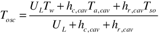
Simplifying yields the bottom insulation other side
condition temperature:
The cavity air temperature is determined from cavity air
heat balance as follows:

Where
h~r, cav~= linearized radiation coefficient for
underlying surface in the cavity, (W/m2K)
h~c, cav~= convection coefficient for underlying
surface in the cavity, (W/m2K)
Tso= the outside face temperature of
the underlying heat transfer surface, (ºC)
 = air mass flow rate due
to natural ventilation, (kg/s)
= air mass flow rate due
to natural ventilation, (kg/s)
qcond= conduction heat flux though the
insulation bottom and, (W/m2)
qconv,cav= convection heat flux between
the collector bottom outside surface and the cavity air,
(W/m2)
qrad,cav=longwave radiation exchange
flux between the collector bottom outside surface and the
outside surface of the underlying surface,
(W/m2)
The cavity air temperature is determined from the cavity
air energy balance. The air heat balance requires the
ventilated cavity air natural ventilation rates. The
calculation of the ventilation rate is described else where in
this document. The SurfaceProperty:ExteriorNaturalVentedCavity,
object is required to describe the surface properties, the
characteristics of the cavity and opening for natural
ventilation.
Heat Transfer
Coefficients[LINK]
The equations used to determine for the various heat
transfer coefficients in the absorber and water heat balance
equations are given below. The absorbed solar energy is
transferred to the water by convection. Assuming natural
convection dominated heat transfer for a hot surface facing
down and a clod surface facing down the following correlation
for Nusselt number by Fujii and Imura (1972). The Nusselt
number for hot surface facing down ward is given by:
The Nusselt number for hot surface upward and cold surface
facing down is given by:
 ****
****
 ****
****
 ****
****
Where,
 = angle of inclination of
the collector to the vertical, radians
= angle of inclination of
the collector to the vertical, radians
g = gravitation force constant, 9.806
(m/s2)
Tr= reference properties where the
thermo-physical properties are calculated, (°C)
Lc= characteristic length for the
absorber plate, (m)
k= thermal conductivity of water at reference
temperature, (W/mK)
= kinematic viscosity of water at reference
temperature, (m2/s)
= thermal diffusivity of water at reference
temperature, (m2/s)
βv= volumetric expansion coefficient
evaluated at Tv, Tv =Tw+0.25(Tp-Tw), (K-1)
Nu= Nusselt number calculated for water properties
at the reference temperature, (-)
Gr= Grashof number calculated for water properties
at the reference temperature, (-)
Pr= Prandtle number calculated for water
properties at the reference temperature, (-)
The various radiation and convection heat transfer
coefficients are given by the following equations. The
convection heat transfer coefficients between the covers and
the absorber plate are estimated from the empirical
correlation for the Nusselt number for air gap between two
parallel plates developed by Hollands et al. (1976) is:


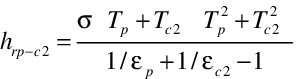

The long wave radiation exchange coefficients between the
outer collector cover and the sky and ground referencing the
ambient air temperature for mathematical simplification are
given.


The convection heat transfer coefficient from the outer
cover to the surrounding air is given by:

When the bottom surface boundary condition is AmbientAir,
the combined conductance from the outer cover to the
surrounding is calculated from the equation below (Duffie and
Beckman, 1991).

The overall loss coefficient through the bottom and side of
the collector-storage is estimated as follows:
Where,
c1 = thermal emissivity of collector
cover 1, (-)
c2 = thermal emissivity of collector
cover 2, (-)
Fs = view factor from the collector to
the sky, (-)
Fg = view factor from the collector to
the ground, (-)
Tc1 = temperature of collector cover
1, (K)
Tc2 = temperature of collector cover
2, (K)
Ts = sky temperature, (K)
Tg= ground temperature, (K)
k = thermal conductivity of air, (W/m K)
L = air gap between the covers, (m)
β = inclination of the plates or covers to the
horizontal, (radian)
Vw = wind speed, (m/s)
ULb= user specified bottom heat loss
conductance, W/m2K
ULs= user specified side heat loss
conductance, W/m2K
Ab= collector bottom heat transfer
area, m2
As= collector side area,
m2
hcomb= combined conductance from the
outer cover to the ambient air, W/m2K
Transmittance-Absorptance Product
The transmittance-absorptance product of solar collector is
determined using ray tracing method for any incident angle
(Duffie and Beckman, 1991). This requires optical properties
of the cover and absorber materials and the the
transmittance-absorptance product for any incident angle is
given by:
The transmittance of the cover system for single and two
cover are given by:
The effective transmittance, reflectance and absorptance of
a single cover are given by:

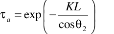
The transmittance of the cover system with absorption only
considered a, is defined as:
The reflectance of un-polarized radiation on passing from
medium 1 with reflective index n1 to
medium 2 with reflective index n2 is given
by:

The sky and ground reflected diffuse radiations average
equivalent incident angles are approximated by Brandemuehl and
Beckman correlation (Duffie and Beckman, 1991) as follows:


where,
**= transmittance of the cover system, (-)
1 = transmittance of the cover 1,
(-)
2 = transmittance of the cover 2,
(-)
**= absorptance of the absorber plate, (-)
d= diffuse reflectance of the inner
cover, (-)
L = thickness of a cover material, (m)
K = extinction coefficient of a cover material,
(m-1)
1 = angle of incidence, degree
2= angle of refraction, degree
 = parallel component of
reflected un-polarized radiation, (-)
= parallel component of
reflected un-polarized radiation, (-)
 = perpendicular component
of reflected un-polarized radiation, (-)
= perpendicular component
of reflected un-polarized radiation, (-)
**= slope of the collector, degree
sd = equivalent incident angle for sky
diffuse solar radiation, degree
gd= equivalent incident angle for
ground diffuse solar radiation, degree
The integral collector storage unit thermal performance
parameters are calculated as follows:
Duffie, J.A., and W.A. Beckman. 1991. Solar Engineering
of Thermal Processes, 2d ed. New York: John Wiley &
Sons.
Kumar, R. and M.A. Rosen. Thermal performance of integrated
collector storage solar water heater with corrugated absorber
surface. Applied Thermal Engineering: 30 (2010) 1764–1768.
Fujii, T., and H. Imura. Natural convection heat transfer
from aplate with arbitrary inclination. International Journal
of Heat and Mass Transfer: 15(4), (1972), 755-764.
Photovoltaic
Thermal Flat-Plate Solar Collectors[LINK]
Photovoltaic-Thermal solar collectors (PVT) combine solar
electric cells and thermal working fluid to collect both
electricity and heat. Athough there are currently
comparatively few commercial products, PVT research has been
conducted for the past 30 years and many different types of
collectors have been studied. Zondag (2008) and Charalambous
et. al (2007) provide reviews of the PVT literature. Because
PVT is much less commercially-mature, there are no standards
or rating systems such as for thermal-only, hot-water
collectors. EnergyPlus currently has one simple model based on
user-defined efficiencies but a more detailed model based on
first-principles and a detailed, layer-by-layer description is
under development.
The PVT models reuse the PV models for electrical
production. These are described elsewhere in this document in
the section on Photovoltaic Arrays-Simple Model
Simple PVT Thermal
Model[LINK]
The input object SolarCollector:FlatPlate:PhotovoltaicThermal
provides a simple PVT model that is provided for quick use
during design or policy studies. The user simply provides
values for a thermal efficiency and the incident solar heats
the working fuild. The model also includes a cooling mode for
air-based systems where a user-provided surface emmittance is
used to model cooling of the working fluid to the night sky
(water-based cooling will be made available once a chilled
water storage tank is available). No other details of the PVT
collector’s construction are required as input data.
The simple model can heat either air or liquid. If it heats
air, then the PVT is part of HVAC air system loop with air
nodes connected to an air system. If it heats liquid, then the
PVT is part of plant loop with nodes connected to a plant loop
and the plant operating scheme determines flows.
Air-system-based PVT modeling include a modulating bypass
damper arrangement. Control logic decides if the air should
bypass the collector to better meet setpoint. The model
requires a drybulb temperature setpoint be placed on the
outlet node. The model assume the collector is intended and
available for heating when the incident solar is greater than
0.3 W/m2 and otherwise it is intended for cooling.
The inlet temperature is compare to the setpoint on the outlet
node to determine if cooling or heating are beneficial. If
they are, then the PVT thermal models are applied to condition
the air stream. If they are not beneficial, then the PVT is
completely bypassed and the inlet node is passed directly to
the outlet node to model a completely bypassed damper
arrangement. A report variable is available for bypass damper
status.
Plant-based PVT do not include a bypass (although one could
be used in the plant loop). The collector requests its design
flow rate but it otherwise relies on the larger plant loop for
control.
When the PVT themal collector is controlled to be “on,” in
heating mode, and working fluid is flowing, the model
calculates the outlet temperature based on the inlet
temperature and the collected heat using the following
equations.
where,
 is the thermal energy
collected [W]
is the thermal energy
collected [W]
 is the net area of the
surface [m2]
is the net area of the
surface [m2]
 is the fraction of
surface aire with active PV/T collector, and
is the fraction of
surface aire with active PV/T collector, and
 is the thermal conversion
efficiency.
is the thermal conversion
efficiency.
where,
 is the temperature of the
working fluid leaving the PV/T
is the temperature of the
working fluid leaving the PV/T
 is the temperature of the
working fluid entering the PV/T
is the temperature of the
working fluid entering the PV/T
 is the entire mass flow
of the working fluid through the PV/T
is the entire mass flow
of the working fluid through the PV/T
 is the specific heat of
the working fluid.
is the specific heat of
the working fluid.
For air-based systems, the value of is then compared to the
temperature setpoint on the outlet node. If exceeds the desired outlet
temperature,  ,then a bypass
fraction is calculated to model a modulating bypass damper
using:
,then a bypass
fraction is calculated to model a modulating bypass damper
using:
When the PVT themal collector is controlled to be “on,” in
cooling mode, and working fluid is flowing, the model
calculates the outlet temperature based on the inlet
temperature and the heat radiated and convected to the ambient
using a heat balance on the outside face of the collector:
Where,
 is the net rate of long
wavelength (thermal) radiation exchange with the air, night
sky, and ground. See the section “External Longwave Radiation”
in the Outside Surface Heat Balance, for full discussion of
how this modeled in EnergyPlus using linearized radiation
coefficients.
is the net rate of long
wavelength (thermal) radiation exchange with the air, night
sky, and ground. See the section “External Longwave Radiation”
in the Outside Surface Heat Balance, for full discussion of
how this modeled in EnergyPlus using linearized radiation
coefficients.
 is the net rate of
convective flux exchange with outdoor air. See the section
“Exterior/External Convection” in the Outside Surface Heat
Balance, for full discussion of how this modeled in
EnergyPlus. The surface roughness is assumed to be “very
smooth.”
is the net rate of
convective flux exchange with outdoor air. See the section
“Exterior/External Convection” in the Outside Surface Heat
Balance, for full discussion of how this modeled in
EnergyPlus. The surface roughness is assumed to be “very
smooth.”
The simple model assumes that the effective collector
temperature,  , is the
average of the working fluid inlet and outlet temperatures so
that we can make the following substitution:
, is the
average of the working fluid inlet and outlet temperatures so
that we can make the following substitution:
Substituting and solving for  we obtain the following model for
collector temperatures during a (possible) cooling process
:
we obtain the following model for
collector temperatures during a (possible) cooling process
:
Then the outlet temperature can be calculated and heat
losses determined. However, the model allows only sensible
cooling of the air stream and limits the outlet temperature to
not go below the dewpoint temperature of the inlet.
PVT collectors have a design volume flow rate for the
working fluid that is autosizable. For air-based systems used
as pre-conditioners, the volume flow rate is sized to meet the
maximum outdoor air flow rate. For water-based systems on the
supply side of a plant loop, each of the PVT collectors are
sized to the overall loop flow rate. For water-based systems
on the demand side of a plant loop, the collectors are sized
using a rule-of-thumb for typical flow rates per unit of
collector area. This rule-of-thumb is based on a constant
factor of 1.905x10⁻⁵
m3/s-m2^^that was developed by analyzing
SRCC data set for conventional solar collectors (see data set
SolarCollectors.idf) and averaging the ratio for all 171
different collectors.
Charalambous, P.G., Maidment, G.G., Kalagirou, S.A., and
Yiakoumetti, K., Photovoltaic thermal (PV/T) collectors: A
review. Applied Thermal Engineering 27 (2007) 275-286.
Zondag, H.A. 2008. Flat-plate PV-Thermal collectors and
systems: A review. Renewable and Sustainable Energy Reviews 12
(2008) 891-959.
Unglazed
Transpired Solar Collectors[LINK]
The input object SolarCollector:UnglazedTranspired
provides a model for transpired collectors that are perhaps
one of the most efficient ways to collect solar energy with
demonstrated instantaneous efficiencies of over 90% and
average efficiencies of over 70%. They are used for preheating
outdoor air needed for ventilation and processes such as crop
drying.
In EnergyPlus, an unglazed transpired solar collector
(UTSC) is modeled as a special component attached to the
outside face of a heat transfer surface that is also connected
to the outdoor air path. A UTSC affects both the thermal
envelope and the HVAC air system. From the air system’s point
of view, a UTSC is heat exchanger and the modeling needs to
determine how much the device raises the temperature of the
outdoor air. From the thermal envelope’s point of view, the
presence of the collector on the outside of the surface
modifies the conditions experienced by the underlying heat
transfer surfaces. EnergyPlus models building performance
throughout the year and the UTSC will often be “off” in terms
of forced airflow, but the collector is still present. When
the UTSC is “on” there is suction airflow that is assumed to
be uniform across the face. When the UTSC is “off” the
collector acts as a radiation and convection baffle situated
between the exterior environment and the outside face of the
underlying heat transfer surface. We distinguish these two
modes of operation as active or passive and
model the UTSC component differently depending on which of
these modes it is in.
Heat Exchanger
Effectiveness[LINK]
The perforated absorber plate is treated as a heat
exchanger and modeled using a traditional effectiveness
formulation. The heat exchanger effectiveness,  , is determined from correlations
derived from small-scale experiments. Two correlations
available in the literature are implemented in EnergyPlus. The
first is based on research by Kutscher at the National
Renewable Energy Laboratory. The second is based on the
research by Van Decker, Hollands, and Brunger at the
University of Waterloo. Because both correlations are
considered valid, the choice of which correlation to use is
left to the user.
, is determined from correlations
derived from small-scale experiments. Two correlations
available in the literature are implemented in EnergyPlus. The
first is based on research by Kutscher at the National
Renewable Energy Laboratory. The second is based on the
research by Van Decker, Hollands, and Brunger at the
University of Waterloo. Because both correlations are
considered valid, the choice of which correlation to use is
left to the user.
Kutscher Correlation[LINK]
Kutscher’s (1994) correlation encompasses surface
convection between the collector and the incoming outdoor air
stream that occurs on the front face, in the holes, and along
the back face of the collector. The correlation uses a
Reynolds number based on the hole diameter as a length scale
and the mean velocity of air as it passes through the holes as
the velocity scale:
where,
 is the velocity through
the holes [m/s]
is the velocity through
the holes [m/s]
 is the hole diameter
[m]
is the hole diameter
[m]
 is the kinematic
viscosity of air [m2/s]
is the kinematic
viscosity of air [m2/s]
The correlation is a function of Reynolds number, hole
geometry, the free stream air velocity, and velocity through
the holes:
where,
 is the pitch, or distance
between holes, [m],
is the pitch, or distance
between holes, [m],
is the diameter of the
holes, [m],
 is the porosity, or area
fraction of the holes, [dimensionless],
is the porosity, or area
fraction of the holes, [dimensionless],
is the mean velocity of
air passing through the holes, [m/s],
 is the free stream
velocity (local wind speed) [m/s].
is the free stream
velocity (local wind speed) [m/s].
The Nusselt number is formulated as:
where,
 is the overall heat
transfer coefficient based on log mean temperature difference,
[W/m2·K], and
is the overall heat
transfer coefficient based on log mean temperature difference,
[W/m2·K], and
 is the thermal
conductivity of air [W/m·K].
is the thermal
conductivity of air [W/m·K].
The heat exchanger effectiveness is:
Kutscher’s relation was formulated for triangular hole
layout, but based on Van Decker et al. (2001) we allow using
the correlation for square hole layout and scale by a factor of 1.6.
Van
Decker, Hollands, and Brunger Correlation[LINK]
Van Decker et. al. extended Kutscher’s measurements to
include a wider range of collector parameters including plate
thickness, pitch, suction velocities, and square hole
patterns. Their model formulation differs from Kutscher’s in
that the model was built up from separate effectiveness models
for the front, back, and holes of the collector. Their
published correlation is:
where,
 is the average suction
velocity across the front face of the collector [m/s]
is the average suction
velocity across the front face of the collector [m/s]
 is the collector plate
thickness
is the collector plate
thickness
Heat Exchanger
Leaving Temperature[LINK]
Using either of the correlations above allows determining
the heat exchanger effectiveness from known values. By
definition the heat exchanger effectiveness is also:
where,
 is the temperature of the
air leaving the collector and entering the plenum [ºC]
is the temperature of the
air leaving the collector and entering the plenum [ºC]
 is the temperature of the
collector’s absorber plate, [ºC], and
is the temperature of the
collector’s absorber plate, [ºC], and
 is the temperature of the
ambient outdoor air [ºC].
is the temperature of the
ambient outdoor air [ºC].
By rewriting equation to solve for we see that the temperature of
the heated outdoor air entering the plenum can be determined
once the collector surface temperature is known,
Collector Heat Balance[LINK]
The collector is assumed to be sufficiently thin and
high-conductivity so that it can be modeled using a single
temperature (for both sides and along its area). This
temperature is determined by
formulating a heat balance on a control volume that just
encapsulates the collector surface. The heat balances are
formulated separately for active and passive modes and are
diagrammed in the following figure.
Observe that for the passive case, we do not use the heat
exchanger relations to directly model the interaction of
ventilating air with the collector. This is because these
relations are considered to not apply when the UTSC is in
passive mode. They were developed for uni-directional flow
(rather than the balanced-in-and-out flow expected from
natural forces) and for specific ranges of suction face
velocity. Therefore, this heat transfer mechanism is handled
using classical surface convection models (as if the collector
was not perforated). (Air exchanges are modeled as ventilation
in the plenum air heat balance but do not interact with the
hole edges in the collector surface.)
When the UTSC is active, the heat balance on the collector
surface control volume is:
where:
 ~~is absorbed direct and
diffuse solar (short wavelength) radiation heat flux.
~~is absorbed direct and
diffuse solar (short wavelength) radiation heat flux.
 is net long wavelength
(thermal) radiation flux exchange with the air and
surroundings.
is net long wavelength
(thermal) radiation flux exchange with the air and
surroundings.
 is surface convection
flux exchange with outdoor air under high wind and rain
conditions. Note that this term is usually assumed to be zero
in UTSC model development but we add the term to allow for
deteriorated performance of the UTSC under poor
conditions.
is surface convection
flux exchange with outdoor air under high wind and rain
conditions. Note that this term is usually assumed to be zero
in UTSC model development but we add the term to allow for
deteriorated performance of the UTSC under poor
conditions.
 ~~is heat exchanger flux
from collector to incoming outdoor air.
~~is heat exchanger flux
from collector to incoming outdoor air.
 ~~is net long wavelength
(thermal) radiation flux exchange with the outside face of the
underlying surface(s).
~~is net long wavelength
(thermal) radiation flux exchange with the outside face of the
underlying surface(s).
 is a source/sink term
that accounts for energy exported out of the control volume
when the collecter’s absorber plate is a hybrid device such as
a photovoltaic panel.
is a source/sink term
that accounts for energy exported out of the control volume
when the collecter’s absorber plate is a hybrid device such as
a photovoltaic panel.
While the heat balance on the passive collector surface
control volume is:
where:
 ~~= surface convection
flux exchange with outdoor air.
~~= surface convection
flux exchange with outdoor air.
 ~~= surface convection
flux exchange with plenum air.
~~= surface convection
flux exchange with plenum air.
All terms are positive for net flux to the collector except
the heat exchanger term, which is taken to be positive in the
direction from collector to incoming air stream. Each of these
heat balance components is introduced briefly below.
External SW Radiation[LINK]
 ~~ is calculated using
procedures presented elsewhere in this manual and includes
both direct and diffuse incident solar radiation absorbed by
the surface face. This is influenced by location, surface
facing angle and tilt, shading surfaces, surface face material
properties, weather conditions, etc.
~~ is calculated using
procedures presented elsewhere in this manual and includes
both direct and diffuse incident solar radiation absorbed by
the surface face. This is influenced by location, surface
facing angle and tilt, shading surfaces, surface face material
properties, weather conditions, etc.
External LW Radiation[LINK]
 is a standard radiation
exchange formulation between the surface, the sky, the ground,
and the atmosphere. The radiation heat flux is calculated from
the surface absorptivity, surface temperature, sky, air, and
ground temperatures, and sky and ground view factors.
Radiation is modeled using linearized coefficients.
is a standard radiation
exchange formulation between the surface, the sky, the ground,
and the atmosphere. The radiation heat flux is calculated from
the surface absorptivity, surface temperature, sky, air, and
ground temperatures, and sky and ground view factors.
Radiation is modeled using linearized coefficients.
External Convection[LINK]
 ~~is modeled using the
classical formulation:
~~is modeled using the
classical formulation:  ~~=
hco(Tair - To) where
hco, is the convection coefficient. This
coefficient will differ depending on whether or not the UTSC
is active or passive. When the UTSC is passive, hco
is treated in the same way as an outside face with
ExteriorEnvironment conditions. When the UTSC is active, the
special suction airflow situation of a transpired collector
during operation means that hcois often zero
because the suction situation can eliminate mass transport
away from the collector. However when the winds are high, the
strong turbulence and highly varying pressures can cause the
suction flow situation to breakdown. Therefore, we include the
~~=
hco(Tair - To) where
hco, is the convection coefficient. This
coefficient will differ depending on whether or not the UTSC
is active or passive. When the UTSC is passive, hco
is treated in the same way as an outside face with
ExteriorEnvironment conditions. When the UTSC is active, the
special suction airflow situation of a transpired collector
during operation means that hcois often zero
because the suction situation can eliminate mass transport
away from the collector. However when the winds are high, the
strong turbulence and highly varying pressures can cause the
suction flow situation to breakdown. Therefore, we include the
 term in the heat balance and
use a special coefficient
term in the heat balance and
use a special coefficient  to
model this lost heat transfer. In addition, when it is raining
outside, we assume the collector gets wet and model the
enhanced surface heat transfer using a large value for .
to
model this lost heat transfer. In addition, when it is raining
outside, we assume the collector gets wet and model the
enhanced surface heat transfer using a large value for .
Heat Exchanger[LINK]
 ~~is modeled using the
classical formulation
~~is modeled using the
classical formulation  ~~where is determined using
correlations described above. When the UTSC is active, the air
mass flow is determined from the operation of the outdoor air
mixer component. When the UTSC is off, this term is zero.
~~where is determined using
correlations described above. When the UTSC is active, the air
mass flow is determined from the operation of the outdoor air
mixer component. When the UTSC is off, this term is zero.
Plenum LW Radation[LINK]
 is a standard radiation
exchange formulation between the collector surface and the
underlying heat transfer surface located across the plenum.
Radiation is modeled using linearized coefficients.
is a standard radiation
exchange formulation between the collector surface and the
underlying heat transfer surface located across the plenum.
Radiation is modeled using linearized coefficients.
Plenum Convection[LINK]
 ~~is modeled using the
classical formulation:
~~is modeled using the
classical formulation:  ~~=
hcp(Tair - To) where
hcp, is the convection coefficient. This
coefficient is taken as zero when the UTSC is operating
because of the suction airflow situation. When the UTSC is
off, the value for hcp is obtained from
correlations used for window gaps from ISO (2003) standard
15099.
~~=
hcp(Tair - To) where
hcp, is the convection coefficient. This
coefficient is taken as zero when the UTSC is operating
because of the suction airflow situation. When the UTSC is
off, the value for hcp is obtained from
correlations used for window gaps from ISO (2003) standard
15099.
Substituting models into and solving for yields the following equation
when the UTSC is active (“on”):
and substituting into yields the following equation when
the UTSC is passive (“off”):
where,
 is the incident solar
radiation of all types [W/m2],
is the incident solar
radiation of all types [W/m2],
 is the solar absorptivity
of the collector [dimensionless],
is the solar absorptivity
of the collector [dimensionless],
 is the linearized
radiation coefficient for the surrounding atmosphere
[W/m2·K],
is the linearized
radiation coefficient for the surrounding atmosphere
[W/m2·K],
 is the outdoor drybulb
from the weather data, also assumed for ground surface
[ºC],
is the outdoor drybulb
from the weather data, also assumed for ground surface
[ºC],
 is the linearized
radiation coefficient for the sky [W/m2·K],
is the linearized
radiation coefficient for the sky [W/m2·K],
 is the effective sky
temperature [ºC],
is the effective sky
temperature [ºC],
 is the linearized
radiation coefficient for the ground [W/m2·K],
is the linearized
radiation coefficient for the ground [W/m2·K],
 is the linearized
radiation coefficient for the underlying surface
[W/m2·K],
is the linearized
radiation coefficient for the underlying surface
[W/m2·K],
is the convection
coefficient for the outdoor environment when the UTSC is
active and winds are high or it is raining
[W/m2·K],
 is the temperature of the
outside face of the underlying heat transfer surface [ºC],
is the temperature of the
outside face of the underlying heat transfer surface [ºC],
 is the air mass flow rate
when in active mode [kg/s],
is the air mass flow rate
when in active mode [kg/s],
 is the specific heat of
air at constant pressure [J/kg·K],
is the specific heat of
air at constant pressure [J/kg·K],
 is the area of the
collector [m2],
is the area of the
collector [m2],
 is the convection
coefficient for the outdoor environment
[W/m2·K],
is the convection
coefficient for the outdoor environment
[W/m2·K],
 is the convection
coefficient for the surfaces facing the plenum
[W/m2·K], and
is the convection
coefficient for the surfaces facing the plenum
[W/m2·K], and
 is the air drybulb for
air in the plenum and entering the outdoor air system
[ºC].
is the air drybulb for
air in the plenum and entering the outdoor air system
[ºC].
Plenum Heat Balance[LINK]
The plenum is the volume of air located between
the collector and the underlying heat transfer surface. The
plenum air is modeled as well-mixed. The uniform temperature
of the plenum air, , is
determined by formulating a heat balance on a control volume
of air as diagrammed below.
Note that we have formulated the control volumes with
slight differences for the active and passive cases. For the
active case, the suction air situation and heat exchanger
effectiveness formulations dictate that the collector surface
control volume encompass part of the air adjacent to both the
front and back surfaces of the collector. However for the
passive case, the collector surface control volume has no air
in it and the plenum air control volume extends all the way to
the surface of the collector.
When the UTSC is active, the heat balance on the plenum air
control volume is:
where,
 is the net rate of energy
added by suction air convecting through the control
volume.
is the net rate of energy
added by suction air convecting through the control
volume.
 ~~ is the net rate of
energy added by surface convection heat transfer with the
underlying surface.
~~ is the net rate of
energy added by surface convection heat transfer with the
underlying surface.
When the UTSC is passive, the heat balance on the plenum
air control volume is:
where,
 is the net rate of energy
added from infiltration – where outdoor ambient air exchanges
with the plenum air.
is the net rate of energy
added from infiltration – where outdoor ambient air exchanges
with the plenum air.
 is the net rate of energy
added by surface convection heat transfer with the
collector.
is the net rate of energy
added by surface convection heat transfer with the
collector.
Substituting into and solving for yields the following equation for
when the UTSC is active:
And substituting into yields the following equation when
the UTSC is passive:
where,
 is the air mass flow from
natural forces [kg/s]
is the air mass flow from
natural forces [kg/s]
The literature on UTSC does not appear to address the
passive mode of operation and no models for  have been identified.
Nevertheless, natural buoyancy and wind forces are expected to
drive air exchange between the plenum and ambient and some
method of modeling
have been identified.
Nevertheless, natural buoyancy and wind forces are expected to
drive air exchange between the plenum and ambient and some
method of modeling  is
needed. Reasoning that the configuration is similar to
single-side natural ventilation, we elect to use correlations
for natural ventilation presented in Chapter 26. of ASHRAE HOF
(2001).
is
needed. Reasoning that the configuration is similar to
single-side natural ventilation, we elect to use correlations
for natural ventilation presented in Chapter 26. of ASHRAE HOF
(2001).
where,
 is the density of air
[kg/m3], and
is the density of air
[kg/m3], and
 is the total volumetric
flow rate of air ventilating in and out of the plenum.
is the total volumetric
flow rate of air ventilating in and out of the plenum.
 (if
(if  )
)
 (if
(if  and UTSC vertical)
 is the effectiveness of
the openings that depends on opening geometry and the
orientation with respect to the wind. ASHRAE HoF (2001)
indicates values ranging from 0.25 to 0.6. In the UTSC model,
this value is available for user input and defaulted to
0.25.
is the effectiveness of
the openings that depends on opening geometry and the
orientation with respect to the wind. ASHRAE HoF (2001)
indicates values ranging from 0.25 to 0.6. In the UTSC model,
this value is available for user input and defaulted to
0.25.
 is the discharge
coefficient for the opening and depends on opening geometry.
In the UTSC model, this value is available for user input and
defaulted to 0.65.
is the discharge
coefficient for the opening and depends on opening geometry.
In the UTSC model, this value is available for user input and
defaulted to 0.65.
Mass continuity arguments lead to modeling the area of the
openings as one half of the total area of the holes, so we
have:
 is the gravitational
constant taken as 9.81 [m/s2].
is the gravitational
constant taken as 9.81 [m/s2].
 is the height from
midpoint of lower opening to the Neutral Pressure Level. This
is taken as one-fourth the overall height of the UTSC if it is
mounted vertically. For tilted collectors, the nominal height
is modified by the sine of the tilt. If the UTSC is mounted
horizontally (e.g. on the roof) then the
is the height from
midpoint of lower opening to the Neutral Pressure Level. This
is taken as one-fourth the overall height of the UTSC if it is
mounted vertically. For tilted collectors, the nominal height
is modified by the sine of the tilt. If the UTSC is mounted
horizontally (e.g. on the roof) then the  is taken as the gap thickness of
the plenum.
is taken as the gap thickness of
the plenum.
If the UTSC is horizontal and  then
then  because this is a stable
situation.
because this is a stable
situation.
Underlying Heat
Transfer Surface[LINK]
The UTSC is applied to the outside of a heat transfer
surface. This surface is modeled using the usual EnergyPlus
methods for handling heat capacity and transients – typically
the CTF method. These native EnergyPlus Heat Balance routines
are used to calculate . The
UTSC model is coupled to the underlying surface using the
OtherSideConditionsModel mechanism. The UTSC model provides
values for , , , and for use with the Heat Balance
Model calculations for the outside face of the underlying
surface (described elsewhere in this manual).
Solar and Shading
Calculations[LINK]
The transpired collector object uses a standard EnergyPlus
surface in order to take advantage of the detailed solar and
shading calculations. Solar radiation incident on the surface
includes beam and diffuse radiation, as well as radiation
reflected from the ground and adjacent surfaces. Shading of
the collector by other surfaces, such as nearby buildings or
trees, is also taken into account.
Local Wind Speed
Calculations[LINK]
The outdoor wind speed affects terms used in modeling UTSC
components. The wind speed in the weather file is assumed to
be measured at a meteorological station located in an open
field at a height of 10 m. To adjust for different terrain at
the building site and differences in the height of building
surfaces, the local wind speed is calculated for each
surface.
The wind speed is modified from the measured meteorological
wind speed by the equation (ASHRAE 2001):
where z is the height of the centroid of the UTSC,
zmet is the height of the standard metereological
wind speed measurement, and a and are terrain-dependent
coefficients. is the boundary layer thickness for the given
terrain type. The values of a and are shown in the following
tables:
Terrain-Dependent Coefficients (ASHRAE
2001).
| Terrain |
Description |
Exponent,
a |
Layer Thickness,
(m) |
| 1 |
Flat, open country |
0.14 |
270 |
| 2 |
Rough, wooded country |
0.22 |
370 |
| 3 |
Towns and cities |
0.33 |
460 |
| 4 |
Ocean |
0.10 |
210 |
| 5 |
Urban, industrial,
forest |
0.22 |
370 |
The UTSC can be defined such that it has multiple
underlying heat transfer surfaces. The centroid heights for
each surface are area-weighted to determine the average height
for use in the local wind calculation.
Convection Coefficients[LINK]
UTSC modeling requires calculating up to three different
coefficients for surface convection heat transfer. These
coefficients are defined in the classic way by:
First, is the convection
coefficient for the collector surface facing the outdoors when
the UTSC is passive. It is modeled in exactly the same way as
elsewhere in EnergyPlus and will depend on the user setting
for Outside Convection Algorithm – Outside Surface Heat
Balance entry elsewhere in this document.
Second, is the convection
coefficient for surfaces facing the plenum. This coefficient
is applied to just the underlying surface’s convection when
the UTSC is active and to both the collector and the
underlying surface when the UTSC is passive. When the UTSC is
active, we use the convection correlation for forced air
developed by McAdams (1954) as published by ASHRAE HoF
(2001):
where,
 is the mean velocity in
the plenum determined from
is the mean velocity in
the plenum determined from  where
where  is the effective cross
section area of the plenum perpendicular to the primary flow
direction. When the UTSC is passive, we model the convection
in the same way used in EnergyPlus to model air gaps in
windows. These correlations vary by Rayleigh number and
surface tilt and are based on the work of various research
including Hollands et. al., Elsherbiny et. al., Wright, and
Arnold. The formulations are documented in ISO (2003) standard
15099. For the UTSC implementation, the routines were adapted
from Subroutine NusseltNumber in WindowManager.f90 (by F.
Winkelmann), which itself was derived from Window5 subroutine
“nusselt”.
is the effective cross
section area of the plenum perpendicular to the primary flow
direction. When the UTSC is passive, we model the convection
in the same way used in EnergyPlus to model air gaps in
windows. These correlations vary by Rayleigh number and
surface tilt and are based on the work of various research
including Hollands et. al., Elsherbiny et. al., Wright, and
Arnold. The formulations are documented in ISO (2003) standard
15099. For the UTSC implementation, the routines were adapted
from Subroutine NusseltNumber in WindowManager.f90 (by F.
Winkelmann), which itself was derived from Window5 subroutine
“nusselt”.
Third, is the convection
coefficient used to degrade the UTSC performance under
environmental conditions with high wind or rain. If the
weather file indicates it is raining, then we set = 1000.0 which has the effect of
making the collector the same temperature as ambient air. The
heat exchanger effectiveness correlations described above
account for a moderate amount of wind, but the correlations
appear confined to the range 0 to 5.0 m/s. Therefore we set
equal to zero if  is <= 5.0 m/s. If
  is > 5.0 m/s then we use the
McAdams correlation but with a reduced velocity magnitude:
is > 5.0 m/s then we use the
McAdams correlation but with a reduced velocity magnitude:


Radiation Coefficients[LINK]
UTSC modeling requires calculating up to four different
linearized coefficients for radiation heat transfer. Whereas
radiation calculations usually use temperature raised to the
fourth power, this greatly complicates solving heat balance
equations for a single temperature. Linearized radiation
coefficients have the same units and are used in the same
manner as surface convection coefficients and introduce very
little error for the temperature levels involved.
The radiation coefficient, , is used to model thermal
radiation between the collector surface and the outside face
of the underlying heat transfer surface. We assume a view
factor of unity. It is calculated using:
where,
all temperatures are converted to Kelvin,
 is the Stefan-Boltzmann
constant,
is the Stefan-Boltzmann
constant,
 is the longwave thermal
emmittance of the collector, and
is the longwave thermal
emmittance of the collector, and
 is the longwave thermal
emmittance of the underlying heat transfer surface.
is the longwave thermal
emmittance of the underlying heat transfer surface.
The three other coefficients, , , and are used elsewhere in EnergyPlus
for the outside face surface heat balance and are calculated
in the same manner as equation for UTSC collectors. [This is
accomplished by calling subroutine
InitExteriorConvectionCoeffs in the file
HeatBalanceConvectionCoeffs.f90. ]
Bypass Control[LINK]
The UTSC is assumed to be arranged so that a bypass damper
controls whether or not air is drawn directly from the
outdoors or through the UTSC. The control decision is based on
whether or not it will be beneficial to heat the outdoor air.
There are multiple levels of control including an availability
schedule, whether or not the outdoor air is cooler than the
mixed air setpoint, or whether or not the zone air temperature
is lower than a so-called free heating setpoint.
Sizing Warnings[LINK]
Although the design of the transpired collector is left to
the user, the program issues warnings when the suction airflow
velocity falls outside the range 0.003 to 0.08 m/s.
Overall Efficiency[LINK]
The overall thermal efficiency of the UTSC is a useful
output report and is defined as the ratio of the useful heat
gain of the entire system versus the total incident solar
radiation on the gross surface area of the collector.
where
 is useful heat gain
 is total incident solar
radiation
is total incident solar
radiation
Note that the efficiency  is only defined for
  . This
efficiency includes heat recovered from the underlying wall
and can exceed 1.0.
. This
efficiency includes heat recovered from the underlying wall
and can exceed 1.0.
Collector Efficiency[LINK]
The thermal efficiency of the collector is a useful output
report and is defined as the ratio of the useful heat gain of
the collector fluid versus the total incident solar radiation
on the gross surface area of the collector.
Note that the efficiency  is only defined for
Kutscher, C.F. 1994. Heat exchange effectiveness and
pressure drop for air flow through perforated plates with and
without crosswind. Journal of Heat Transfer. May
1994, Vol. 116, p. 391. American Society of Mechanical
Engineers.
Van Decker, G.W.E., K.G.T. Hollands, and A.P. Brunger.
2001. Heat-exchange relations for unglazed transpired solar
collectors with circular holes on a square of triangular
pitch. Solar Energy. Vol. 71, No. 1. pp 33-45,
2001.
ISO. 2003. ISO 15099:2003. Thermal performance of windows,
doors, and shading devices – Detailed calculations.
International Organization for Standardization.

Solar Collectors[LINK]
Solar collectors are devices that convert solar energy into thermal energy by raising the temperature of a circulating heat transfer fluid. The fluid can then be used to heat water for domestic hot water usage or space heating. Flat-plate solar collectors using water as the heat transfer fluid, Integral-Collector Storage solar collectors using water and unglazed transpired solar collectors using air are currently the only types of collector available in EnergyPlus.
Flat-Plate Solar Collectors[LINK]
The input object SolarCollector:FlatPlate:Water provides a model for flat-plate solar collectors that are the most common type of collector. Standards have been established by ASHRAE for the performance testing of these collectors (ASHRAE 1989; 1991) and the Solar Rating and Certification Corporation (SRCC) publishes a directory of commercially available collectors in North America (SRCC 2003).
The EnergyPlus model is based on the equations found in the ASHRAE standards and Duffie and Beckman (1991). This model applies to glazed and unglazed flat-plate collectors, as well as banks of tubular, i.e. evacuated tube, collectors.
Solar and Shading Calculations[LINK]
The solar collector object uses a standard EnergyPlus surface in order to take advantage of the detailed solar and shading calculations. Solar radiation incident on the surface includes beam and diffuse radiation, as well as radiation reflected from the ground and adjacent surfaces. Shading of the collector by other surfaces, such as nearby buildings or trees, is also taken into account. Likewise, the collector surface can shade other surfaces, for example, reducing the incident radiation on the roof beneath it.
Thermal Performance[LINK]
The thermal efficiency of a collector is defined as the ratio of the useful heat gain of the collector fluid versus the total incident solar radiation on the gross surface area of the collector.
where
q = useful heat gain
A = gross area of the collector
Isolar = total incident solar radiation
Notice that the efficiency is only defined for Isolar > 0.
An energy balance on a solar collector with double glazing shows relationships between the glazing properties, absorber plate properties, and environmental conditions.
where
g1 = transmittance of the first glazing layer
g2 = transmittance of the second glazing layer
abs = absorptance of the absorber plate
Rrad = radiative resistance from absorber to inside glazing
Rconv = convective resistance from absorber to inside glazing
Rcond = conductive resistance from absorber to outdoor air through the insulation
Tabs = temperature of the absorber plate
Tg2 = temperature of the inside glazing
Tair = temperature of the outdoor air
The equation above can be approximated with a simpler formulation as:
where
FR = an empirically determined correction factor
() = the product of all transmittance and absorptance terms
UL = overall heat loss coefficient combining radiation, convection, and conduction terms
Tin = inlet temperature of the working fluid
Substituting this into Equation ,
A linear correlation can be constructed by treating FR() and -FRUL as characteristic constants of the solar collector:
Similarly, a quadratic correlation can be constructed using the form:
Both first- and second-order efficiency equation coefficients are listed in the Directory of SRCC Certified Solar Collector Ratings.
Incident Angle Modifiers[LINK]
As with regular windows the transmittance of the collector glazing varies with the incidence angle of radiation. Usually the transmittance is highest when the incident radiation is normal to the glazing surface. Test conditions determine the efficiency coefficients for normal incidence. For off-normal angles, the transmittance of the glazing is modified by an incident angle modifier coefficient.
Additional testing determines the incident angle modifier as a function of incident angle . This relationship can be fit to a first-order, linear correlation:
or a second-order, quadratic correlation:
The incident angle modifier coefficients b0 and b1 are usually negative, although some collectors have a positive value for b0. Both first- and second-order incident angle modifier equation coefficients are listed in the Directory of SRCC Certified Solar Collector Ratings.
The SRCC incident angle modifier equation coefficients are only valid for incident angles of 60 degrees or less. Because these curves can be valid yet behave poorly for angles greater than 60 degree, the EnergyPlus model cuts off collector gains for incident angles greater than 60 degrees.
For flat-plate collectors, the incident angle modifier is generally symmetrical. However, for tubular collectors the incident angle modifier is different depending on whether the incident angle is parallel or perpendicular to the tubes. These are called bi-axial modifiers. Some special flat-plate collectors may also exhibit this asymmetry. The current model cannot yet handle two sets of incident angle modifiers. In the meantime it is recommended that tubular collectors be approximated with caution using either the parallel or perpendicular correlation.
Incident angle modifiers are calculated separately for sun, sky, and ground radiation. The net incident angle modifier for all incident radiation is calculated by weighting each component by the corresponding modifier.
For sky and ground radiation the incident angle is approximated using Brandemuehl and Beckman’s equations:
where is the surface tilt in degrees.
The net incident angle modifier is then inserted into the useful heat gain equation :
Equation is also modified accordingly.
Outlet Temperature[LINK]
Outlet temperature is calculated using the useful heat gain q as determined by Equation , the inlet fluid temperature Tin, and the mass flow rate available from the plant simulation:
where
cp = specific heat of the working fluid
Solving for Tout,
If there is no flow through the collector, Tout is the stagnation temperature of the fluid. This is calculated by setting the left side of Equation to zero and solving for Tin (which also equals Tout for the no flow case).
References[LINK]
ASHRAE. 1989. ASHRAE Standard 96-1980 (RA 89): Methods of Testing to Determine the Thermal Performance of Unglazed Flat-Plate Liquid-Type Solar Collectors. Atlanta: American Society of Heating, Refrigerating and Air-Conditioning Engineers, Inc.
ASHRAE. 1991. ASHRAE Standard 93-1986 (RA 91): Methods of Testing to Determine the Thermal Performance of Solar Collectors. Atlanta: American Society of Heating, Refrigerating and Air-Conditioning Engineers, Inc.
Duffie, J. A., and Beckman, W. A. 1991. Solar Engineering of Thermal Processes, Second Edition. New York: Wiley-Interscience.
Solar Rating and Certification Corporation. 2004. Directory of SRCC Certified Solar Collector Ratings, OG 100. Cocoa, Florida: Solar Rating and Certification Corporation.
Integral-collector-storage (ICS) Solar Collector[LINK]
Solar collectors with integral storage unit models use SolarCollector:IntegralCollectorStorage object, and the characteristics parameter inputs of this collector are provided by the SolarCollectorPerformance:IntegralCollectorStorage object. This model is based on detailed Energy Balance equations of solar collectors that integrates storage in it. This model has two options to represent the collector bottom outside boundary conditions: AmbientAir, and OtherSideConditionsModel. AmbientAir simply applies outside air temperature using combined convection and radiation conductance, and the OtherSideConditionsModel applies combined radiation and convection models that exiats in a naturally ventilated cavity to represent the collector bottom outside boundary condition. The later boundary condition accounts for the shading of the collector on the underlying surface, hence, the ICS collector can be assumed as an integral part of the building envelope. Schamtic diagram of a rectangular ICS solar collector is shown in Figure 294 below:
Solar and Shading Calculations[LINK]
The solar collector object uses a standard EnergyPlus surface in order to take advantage of the detailed solar and shading calculations. Solar radiation incident on the surface includes beam and diffuse radiation, as well as radiation reflected from the ground and adjacent surfaces. Shading of the collector by other surfaces, such as nearby buildings or trees, is also taken into account. Likewise, the collector surface shades the roof surface beneath it, hence no direct solar radiation incident on the roof surface. The collector and the roof outside boundary conditions should be specified as OtherSideConditionModel to account for solar collector shading impact on the roof surface.
Mathematical Model[LINK]
The integral-collector-storage (ICS) solar collector is represented using two transient energy balance equations shown below. These equations represent the energy balance equation for the absorber plate, and the water in the collector.
Where,
mpCp= thermal capacity of the absorber surface, J/°C
A= collector gross area, m2
()e= transmittance-absorptance product of the absorber plate and cover system
It = total solar irradiation, (W/m2)
hpw= convective heat transfer coefficient from absorber plate to water, (W/m2°K)
Ut= overall heat loss coefficient from absorber to the ambient air, (W/m2 °K)
Tp= absorber plate average temperature, (°C)
Tw= collector water average temperature, (°C)
Ta= ambient air temperature, (°C)
mwCpw = thermal capacity of the water mass in the collector, (J/°C)
Us= area-weighted conductance of the collector side insulation, (W/m2°K)
Ub= conductance of the collector bottom insulation, (W/m2°K)
Tosc=outside temperature of bottom insulation determined from the other side condition model, (°C)
Twi= Entering makeup or mains water temperature, (°C)
The other side condition model boundary condition represented by the Tosc, allows us to apply a realistic outside boundary condition for a collector mounted on a building roof. This also accounts for the shading impact of the collector on the under-laying surface (roof). On the other hand if ambient air boundary condition is specified, then the collector does not shade the underlying surface it is mounted on.
The two energy balance equation can be written as non-homogeneous first order DE with constant coefficients. The initial conditions for these equations are the absorber plate average temperature and the collector water average temperature at previous time steps.
The two coupled first order differential equation are solved analytically. Auxiliary equation of the the coupled homogeneous differential equation is given by:
This auxiliary quadratic equation has always two distinct real roots (1 and 2) hence the solution of the homogeneous equation is exponential, and the general solutions of the differential equations are given by:
The constant terms A and B are the particular solution of the non-homogeneous differential equations, the coefficients of the exponential terms (c1, c2, r1, and r2) are determined from the initial conditions of the absorber and collector water temperatures (Tp0, Tw0) and are given by:
Thermal Network Model:[LINK]
The thermal network model requires energy balance for each of the collector covers as well. The heat balance equation of the collector covers is assumed to obey steady state formulation by ignoring their thermal mass. The thermal-network representation of the ICS collector is shown in Figure 295. Also, the heat balance at each cover surface requires knowledge of the amount of solar fraction absorbed, which is determined from the ray tracing analysis. For the thermal network model shown above the overall top heat loss coefficient is determined from combination of the resistances in series as follows:
Or
The convection and radiation heat transfer coefficients in equation above are calculated based on temperatures at the previous time step and determined as described in the Heat Transfer Coefficients section.
Collector Cover Heat Balance
Ignoring the thermal mass of the collector cover, a steady state heat balance equations are formulated for each cover that allow us to determine cover temperatures. The cover surface heat balance representation is shown in Figure 296 below.
The steady state cover heat balance equation is given by:
Linearizing the longwave radiation exchange and representing the convection terms using the classical equation for Newton’s law of cooling, the equations for the temperatures of covers 1 and 2 are given by:
Where,
c = the weighted average solar absorptance of covers 1 and 2, (-)
hr,c1-a= adjusted radiation heat transfer coefficient between cover 1 and the ambient air, (W/m2K)
hc,c1-a= convection heat transfer coefficient between cover 1 and the ambient, (W/m2K)
hr,c2-c1= radiation heat transfer coefficient between covers 1 and 2, (W/m2K)
hc,c2-c1= convection heat transfer coefficient between covers 1 and 2, (W/m2K)
hr,p-c2= radiation heat transfer coefficient between covers 2 and the absorber plate, (W/m2K)
hc,p-c2= convection heat transfer coefficient between covers 2 and the absorber plate, (W/m2K)
qLWR,1= longwave radiation exchange flux on side 1 of the collector cover, (W/m2)
qCONV,1= convection heat flux on side 1 of the collector cover, (W/m2)
qLWR,2= longwave radiation exchange flux on side 2 of the collector cover, (W/m2)
qCONV,2= convection heat flux on side 2 of the collector cover, (W/m2)
qsolar,abs= net solar radiation absorbed by the collector cover, (W/m2)
R= thermal resistance for each section along the heat flow path, (m2K/W)
Other Side Condition Model[LINK]
ICS Solar Collectors are commonly mounted on building heat transfer surfaces hence the collectors shade the underlying heat transfer surface and require a unique boundary condition that reflects the air cavity environment created between the bottom of the collector surface and the underlying surface. The other side condition model that allows us to estimate the other side temperature, Tosc, can be determined based on steady state heat balance using the known collector water temperature at the previous time step.
Ignoring thermal mass of the collector bottom insulation, steady state surface heat balance can be formulated on the outer plane of the collector bottom surface facing the cavity as shown in Figure 4. The heat balance equation on the outer plane of the collector bottom surface is given by:
Substituting the equations for each term in the above equation yields:
Simplifying yields the bottom insulation other side condition temperature:
The cavity air temperature is determined from cavity air heat balance as follows:
Where
h~r, cav~= linearized radiation coefficient for underlying surface in the cavity, (W/m2K)
h~c, cav~= convection coefficient for underlying surface in the cavity, (W/m2K)
Tso= the outside face temperature of the underlying heat transfer surface, (ºC)
qcond= conduction heat flux though the insulation bottom and, (W/m2)
qconv,cav= convection heat flux between the collector bottom outside surface and the cavity air, (W/m2)
qrad,cav=longwave radiation exchange flux between the collector bottom outside surface and the outside surface of the underlying surface, (W/m2)
The cavity air temperature is determined from the cavity air energy balance. The air heat balance requires the ventilated cavity air natural ventilation rates. The calculation of the ventilation rate is described else where in this document. The SurfaceProperty:ExteriorNaturalVentedCavity, object is required to describe the surface properties, the characteristics of the cavity and opening for natural ventilation.
Heat Transfer Coefficients[LINK]
The equations used to determine for the various heat transfer coefficients in the absorber and water heat balance equations are given below. The absorbed solar energy is transferred to the water by convection. Assuming natural convection dominated heat transfer for a hot surface facing down and a clod surface facing down the following correlation for Nusselt number by Fujii and Imura (1972). The Nusselt number for hot surface facing down ward is given by:
The Nusselt number for hot surface upward and cold surface facing down is given by:
Where,
g = gravitation force constant, 9.806 (m/s2)
Tr= reference properties where the thermo-physical properties are calculated, (°C)
Lc= characteristic length for the absorber plate, (m)
k= thermal conductivity of water at reference temperature, (W/mK)
= kinematic viscosity of water at reference temperature, (m2/s)
= thermal diffusivity of water at reference temperature, (m2/s)
βv= volumetric expansion coefficient evaluated at Tv, Tv =Tw+0.25(Tp-Tw), (K-1)
Nu= Nusselt number calculated for water properties at the reference temperature, (-)
Gr= Grashof number calculated for water properties at the reference temperature, (-)
Pr= Prandtle number calculated for water properties at the reference temperature, (-)
The various radiation and convection heat transfer coefficients are given by the following equations. The convection heat transfer coefficients between the covers and the absorber plate are estimated from the empirical correlation for the Nusselt number for air gap between two parallel plates developed by Hollands et al. (1976) is:
The long wave radiation exchange coefficients between the outer collector cover and the sky and ground referencing the ambient air temperature for mathematical simplification are given.
The convection heat transfer coefficient from the outer cover to the surrounding air is given by:
When the bottom surface boundary condition is AmbientAir, the combined conductance from the outer cover to the surrounding is calculated from the equation below (Duffie and Beckman, 1991).
The overall loss coefficient through the bottom and side of the collector-storage is estimated as follows:
Where,
c1 = thermal emissivity of collector cover 1, (-)
c2 = thermal emissivity of collector cover 2, (-)
Fs = view factor from the collector to the sky, (-)
Fg = view factor from the collector to the ground, (-)
Tc1 = temperature of collector cover 1, (K)
Tc2 = temperature of collector cover 2, (K)
Ts = sky temperature, (K)
Tg= ground temperature, (K)
k = thermal conductivity of air, (W/m K)
L = air gap between the covers, (m)
β = inclination of the plates or covers to the horizontal, (radian)
Vw = wind speed, (m/s)
ULb= user specified bottom heat loss conductance, W/m2K
ULs= user specified side heat loss conductance, W/m2K
Ab= collector bottom heat transfer area, m2
As= collector side area, m2
hcomb= combined conductance from the outer cover to the ambient air, W/m2K
Transmittance-Absorptance Product
The transmittance-absorptance product of solar collector is determined using ray tracing method for any incident angle (Duffie and Beckman, 1991). This requires optical properties of the cover and absorber materials and the the transmittance-absorptance product for any incident angle is given by:
The transmittance of the cover system for single and two cover are given by:
The effective transmittance, reflectance and absorptance of a single cover are given by:
The transmittance of the cover system with absorption only considered a, is defined as:
The reflectance of un-polarized radiation on passing from medium 1 with reflective index n1 to medium 2 with reflective index n2 is given by:
The sky and ground reflected diffuse radiations average equivalent incident angles are approximated by Brandemuehl and Beckman correlation (Duffie and Beckman, 1991) as follows:
where,
**= transmittance of the cover system, (-)
1 = transmittance of the cover 1, (-)
2 = transmittance of the cover 2, (-)
**= absorptance of the absorber plate, (-)
d= diffuse reflectance of the inner cover, (-)
L = thickness of a cover material, (m)
K = extinction coefficient of a cover material, (m-1)
1 = angle of incidence, degree
2= angle of refraction, degree
**= slope of the collector, degree
sd = equivalent incident angle for sky diffuse solar radiation, degree
gd= equivalent incident angle for ground diffuse solar radiation, degree
The integral collector storage unit thermal performance parameters are calculated as follows:
References:[LINK]
Duffie, J.A., and W.A. Beckman. 1991. Solar Engineering of Thermal Processes, 2d ed. New York: John Wiley & Sons.
Kumar, R. and M.A. Rosen. Thermal performance of integrated collector storage solar water heater with corrugated absorber surface. Applied Thermal Engineering: 30 (2010) 1764–1768.
Fujii, T., and H. Imura. Natural convection heat transfer from aplate with arbitrary inclination. International Journal of Heat and Mass Transfer: 15(4), (1972), 755-764.
Photovoltaic Thermal Flat-Plate Solar Collectors[LINK]
Photovoltaic-Thermal solar collectors (PVT) combine solar electric cells and thermal working fluid to collect both electricity and heat. Athough there are currently comparatively few commercial products, PVT research has been conducted for the past 30 years and many different types of collectors have been studied. Zondag (2008) and Charalambous et. al (2007) provide reviews of the PVT literature. Because PVT is much less commercially-mature, there are no standards or rating systems such as for thermal-only, hot-water collectors. EnergyPlus currently has one simple model based on user-defined efficiencies but a more detailed model based on first-principles and a detailed, layer-by-layer description is under development.
The PVT models reuse the PV models for electrical production. These are described elsewhere in this document in the section on Photovoltaic Arrays-Simple Model
Simple PVT Thermal Model[LINK]
The input object SolarCollector:FlatPlate:PhotovoltaicThermal provides a simple PVT model that is provided for quick use during design or policy studies. The user simply provides values for a thermal efficiency and the incident solar heats the working fuild. The model also includes a cooling mode for air-based systems where a user-provided surface emmittance is used to model cooling of the working fluid to the night sky (water-based cooling will be made available once a chilled water storage tank is available). No other details of the PVT collector’s construction are required as input data.
The simple model can heat either air or liquid. If it heats air, then the PVT is part of HVAC air system loop with air nodes connected to an air system. If it heats liquid, then the PVT is part of plant loop with nodes connected to a plant loop and the plant operating scheme determines flows.
Air-system-based PVT modeling include a modulating bypass damper arrangement. Control logic decides if the air should bypass the collector to better meet setpoint. The model requires a drybulb temperature setpoint be placed on the outlet node. The model assume the collector is intended and available for heating when the incident solar is greater than 0.3 W/m2 and otherwise it is intended for cooling. The inlet temperature is compare to the setpoint on the outlet node to determine if cooling or heating are beneficial. If they are, then the PVT thermal models are applied to condition the air stream. If they are not beneficial, then the PVT is completely bypassed and the inlet node is passed directly to the outlet node to model a completely bypassed damper arrangement. A report variable is available for bypass damper status.
Plant-based PVT do not include a bypass (although one could be used in the plant loop). The collector requests its design flow rate but it otherwise relies on the larger plant loop for control.
When the PVT themal collector is controlled to be “on,” in heating mode, and working fluid is flowing, the model calculates the outlet temperature based on the inlet temperature and the collected heat using the following equations.
where,
where,
For air-based systems, the value of is then compared to the
temperature setpoint on the outlet node. If
is then compared to the
temperature setpoint on the outlet node. If  exceeds the desired outlet
temperature,
exceeds the desired outlet
temperature,  ,then a bypass
fraction is calculated to model a modulating bypass damper
using:
,then a bypass
fraction is calculated to model a modulating bypass damper
using:
When the PVT themal collector is controlled to be “on,” in cooling mode, and working fluid is flowing, the model calculates the outlet temperature based on the inlet temperature and the heat radiated and convected to the ambient using a heat balance on the outside face of the collector:
Where,
The simple model assumes that the effective collector temperature, , is the
average of the working fluid inlet and outlet temperatures so
that we can make the following substitution:
, is the
average of the working fluid inlet and outlet temperatures so
that we can make the following substitution:
Substituting and solving for we obtain the following model for
collector temperatures during a (possible) cooling process
:
we obtain the following model for
collector temperatures during a (possible) cooling process
:
Then the outlet temperature can be calculated and heat losses determined. However, the model allows only sensible cooling of the air stream and limits the outlet temperature to not go below the dewpoint temperature of the inlet.
PVT collectors have a design volume flow rate for the working fluid that is autosizable. For air-based systems used as pre-conditioners, the volume flow rate is sized to meet the maximum outdoor air flow rate. For water-based systems on the supply side of a plant loop, each of the PVT collectors are sized to the overall loop flow rate. For water-based systems on the demand side of a plant loop, the collectors are sized using a rule-of-thumb for typical flow rates per unit of collector area. This rule-of-thumb is based on a constant factor of 1.905x10⁻⁵ m3/s-m2^^that was developed by analyzing SRCC data set for conventional solar collectors (see data set SolarCollectors.idf) and averaging the ratio for all 171 different collectors.
References[LINK]
Charalambous, P.G., Maidment, G.G., Kalagirou, S.A., and Yiakoumetti, K., Photovoltaic thermal (PV/T) collectors: A review. Applied Thermal Engineering 27 (2007) 275-286.
Zondag, H.A. 2008. Flat-plate PV-Thermal collectors and systems: A review. Renewable and Sustainable Energy Reviews 12 (2008) 891-959.
Unglazed Transpired Solar Collectors[LINK]
The input object SolarCollector:UnglazedTranspired provides a model for transpired collectors that are perhaps one of the most efficient ways to collect solar energy with demonstrated instantaneous efficiencies of over 90% and average efficiencies of over 70%. They are used for preheating outdoor air needed for ventilation and processes such as crop drying.
In EnergyPlus, an unglazed transpired solar collector (UTSC) is modeled as a special component attached to the outside face of a heat transfer surface that is also connected to the outdoor air path. A UTSC affects both the thermal envelope and the HVAC air system. From the air system’s point of view, a UTSC is heat exchanger and the modeling needs to determine how much the device raises the temperature of the outdoor air. From the thermal envelope’s point of view, the presence of the collector on the outside of the surface modifies the conditions experienced by the underlying heat transfer surfaces. EnergyPlus models building performance throughout the year and the UTSC will often be “off” in terms of forced airflow, but the collector is still present. When the UTSC is “on” there is suction airflow that is assumed to be uniform across the face. When the UTSC is “off” the collector acts as a radiation and convection baffle situated between the exterior environment and the outside face of the underlying heat transfer surface. We distinguish these two modes of operation as active or passive and model the UTSC component differently depending on which of these modes it is in.
Heat Exchanger Effectiveness[LINK]
The perforated absorber plate is treated as a heat exchanger and modeled using a traditional effectiveness formulation. The heat exchanger effectiveness, , is determined from correlations
derived from small-scale experiments. Two correlations
available in the literature are implemented in EnergyPlus. The
first is based on research by Kutscher at the National
Renewable Energy Laboratory. The second is based on the
research by Van Decker, Hollands, and Brunger at the
University of Waterloo. Because both correlations are
considered valid, the choice of which correlation to use is
left to the user.
, is determined from correlations
derived from small-scale experiments. Two correlations
available in the literature are implemented in EnergyPlus. The
first is based on research by Kutscher at the National
Renewable Energy Laboratory. The second is based on the
research by Van Decker, Hollands, and Brunger at the
University of Waterloo. Because both correlations are
considered valid, the choice of which correlation to use is
left to the user.
Kutscher Correlation[LINK]
Kutscher’s (1994) correlation encompasses surface convection between the collector and the incoming outdoor air stream that occurs on the front face, in the holes, and along the back face of the collector. The correlation uses a Reynolds number based on the hole diameter as a length scale and the mean velocity of air as it passes through the holes as the velocity scale:
where,
The correlation is a function of Reynolds number, hole geometry, the free stream air velocity, and velocity through the holes:
where,
The Nusselt number is formulated as:
where,
The heat exchanger effectiveness is:
Kutscher’s relation was formulated for triangular hole layout, but based on Van Decker et al. (2001) we allow using the correlation for square hole layout and scale by a factor of 1.6.
Van Decker, Hollands, and Brunger Correlation[LINK]
Van Decker et. al. extended Kutscher’s measurements to include a wider range of collector parameters including plate thickness, pitch, suction velocities, and square hole patterns. Their model formulation differs from Kutscher’s in that the model was built up from separate effectiveness models for the front, back, and holes of the collector. Their published correlation is:
where,
Heat Exchanger Leaving Temperature[LINK]
Using either of the correlations above allows determining the heat exchanger effectiveness from known values. By definition the heat exchanger effectiveness is also:
where,
By rewriting equation to solve for we see that the temperature of
the heated outdoor air entering the plenum can be determined
once the collector surface temperature is known,
we see that the temperature of
the heated outdoor air entering the plenum can be determined
once the collector surface temperature is known,
Collector Heat Balance[LINK]
The collector is assumed to be sufficiently thin and high-conductivity so that it can be modeled using a single temperature (for both sides and along its area). This temperature is determined by
formulating a heat balance on a control volume that just
encapsulates the collector surface. The heat balances are
formulated separately for active and passive modes and are
diagrammed in the following figure.
is determined by
formulating a heat balance on a control volume that just
encapsulates the collector surface. The heat balances are
formulated separately for active and passive modes and are
diagrammed in the following figure.
Observe that for the passive case, we do not use the heat exchanger relations to directly model the interaction of ventilating air with the collector. This is because these relations are considered to not apply when the UTSC is in passive mode. They were developed for uni-directional flow (rather than the balanced-in-and-out flow expected from natural forces) and for specific ranges of suction face velocity. Therefore, this heat transfer mechanism is handled using classical surface convection models (as if the collector was not perforated). (Air exchanges are modeled as ventilation in the plenum air heat balance but do not interact with the hole edges in the collector surface.)
When the UTSC is active, the heat balance on the collector surface control volume is:
where:
While the heat balance on the passive collector surface control volume is:
where:
All terms are positive for net flux to the collector except the heat exchanger term, which is taken to be positive in the direction from collector to incoming air stream. Each of these heat balance components is introduced briefly below.
External SW Radiation[LINK]
External LW Radiation[LINK]
External Convection[LINK]
Heat Exchanger[LINK]
Plenum LW Radation[LINK]
Plenum Convection[LINK]
Substituting models into and solving for yields the following equation
when the UTSC is active (“on”):
yields the following equation
when the UTSC is active (“on”):
and substituting into yields the following equation when the UTSC is passive (“off”):
where,
Plenum Heat Balance[LINK]
The plenum is the volume of air located between the collector and the underlying heat transfer surface. The plenum air is modeled as well-mixed. The uniform temperature of the plenum air, , is
determined by formulating a heat balance on a control volume
of air as diagrammed below.
, is
determined by formulating a heat balance on a control volume
of air as diagrammed below.
Note that we have formulated the control volumes with slight differences for the active and passive cases. For the active case, the suction air situation and heat exchanger effectiveness formulations dictate that the collector surface control volume encompass part of the air adjacent to both the front and back surfaces of the collector. However for the passive case, the collector surface control volume has no air in it and the plenum air control volume extends all the way to the surface of the collector.
When the UTSC is active, the heat balance on the plenum air control volume is:
where,
When the UTSC is passive, the heat balance on the plenum air control volume is:
where,
Substituting into and solving for yields the following equation for
when the UTSC is active:
yields the following equation for
when the UTSC is active:
And substituting into yields the following equation when the UTSC is passive:
where,
The literature on UTSC does not appear to address the passive mode of operation and no models for have been identified.
Nevertheless, natural buoyancy and wind forces are expected to
drive air exchange between the plenum and ambient and some
method of modeling
have been identified.
Nevertheless, natural buoyancy and wind forces are expected to
drive air exchange between the plenum and ambient and some
method of modeling  is
needed. Reasoning that the configuration is similar to
single-side natural ventilation, we elect to use correlations
for natural ventilation presented in Chapter 26. of ASHRAE HOF
(2001).
is
needed. Reasoning that the configuration is similar to
single-side natural ventilation, we elect to use correlations
for natural ventilation presented in Chapter 26. of ASHRAE HOF
(2001).
where,
Mass continuity arguments lead to modeling the area of the openings as one half of the total area of the holes, so we have:
If the UTSC is horizontal and then
then  because this is a stable
situation.
because this is a stable
situation.
Underlying Heat Transfer Surface[LINK]
The UTSC is applied to the outside of a heat transfer surface. This surface is modeled using the usual EnergyPlus methods for handling heat capacity and transients – typically the CTF method. These native EnergyPlus Heat Balance routines are used to calculate . The
UTSC model is coupled to the underlying surface using the
OtherSideConditionsModel mechanism. The UTSC model provides
values for
. The
UTSC model is coupled to the underlying surface using the
OtherSideConditionsModel mechanism. The UTSC model provides
values for  ,
, ,
,  , and
, and  for use with the Heat Balance
Model calculations for the outside face of the underlying
surface (described elsewhere in this manual).
for use with the Heat Balance
Model calculations for the outside face of the underlying
surface (described elsewhere in this manual).
Solar and Shading Calculations[LINK]
The transpired collector object uses a standard EnergyPlus surface in order to take advantage of the detailed solar and shading calculations. Solar radiation incident on the surface includes beam and diffuse radiation, as well as radiation reflected from the ground and adjacent surfaces. Shading of the collector by other surfaces, such as nearby buildings or trees, is also taken into account.
Local Wind Speed Calculations[LINK]
The outdoor wind speed affects terms used in modeling UTSC components. The wind speed in the weather file is assumed to be measured at a meteorological station located in an open field at a height of 10 m. To adjust for different terrain at the building site and differences in the height of building surfaces, the local wind speed is calculated for each surface.
The wind speed is modified from the measured meteorological wind speed by the equation (ASHRAE 2001):
where z is the height of the centroid of the UTSC, zmet is the height of the standard metereological wind speed measurement, and a and are terrain-dependent coefficients. is the boundary layer thickness for the given terrain type. The values of a and are shown in the following tables:
The UTSC can be defined such that it has multiple underlying heat transfer surfaces. The centroid heights for each surface are area-weighted to determine the average height for use in the local wind calculation.
Convection Coefficients[LINK]
UTSC modeling requires calculating up to three different coefficients for surface convection heat transfer. These coefficients are defined in the classic way by:
First, is the convection
coefficient for the collector surface facing the outdoors when
the UTSC is passive. It is modeled in exactly the same way as
elsewhere in EnergyPlus and will depend on the user setting
for Outside Convection Algorithm – Outside Surface Heat
Balance entry elsewhere in this document.
is the convection
coefficient for the collector surface facing the outdoors when
the UTSC is passive. It is modeled in exactly the same way as
elsewhere in EnergyPlus and will depend on the user setting
for Outside Convection Algorithm – Outside Surface Heat
Balance entry elsewhere in this document.
Second, is the convection
coefficient for surfaces facing the plenum. This coefficient
is applied to just the underlying surface’s convection when
the UTSC is active and to both the collector and the
underlying surface when the UTSC is passive. When the UTSC is
active, we use the convection correlation for forced air
developed by McAdams (1954) as published by ASHRAE HoF
(2001):
is the convection
coefficient for surfaces facing the plenum. This coefficient
is applied to just the underlying surface’s convection when
the UTSC is active and to both the collector and the
underlying surface when the UTSC is passive. When the UTSC is
active, we use the convection correlation for forced air
developed by McAdams (1954) as published by ASHRAE HoF
(2001):
where,
Third, is the convection
coefficient used to degrade the UTSC performance under
environmental conditions with high wind or rain. If the
weather file indicates it is raining, then we set
is the convection
coefficient used to degrade the UTSC performance under
environmental conditions with high wind or rain. If the
weather file indicates it is raining, then we set  = 1000.0 which has the effect of
making the collector the same temperature as ambient air. The
heat exchanger effectiveness correlations described above
account for a moderate amount of wind, but the correlations
appear confined to the range 0 to 5.0 m/s. Therefore we set
= 1000.0 which has the effect of
making the collector the same temperature as ambient air. The
heat exchanger effectiveness correlations described above
account for a moderate amount of wind, but the correlations
appear confined to the range 0 to 5.0 m/s. Therefore we set
 equal to zero if
  is <= 5.0 m/s. If
  is > 5.0 m/s then we use the
McAdams correlation but with a reduced velocity magnitude:
is > 5.0 m/s then we use the
McAdams correlation but with a reduced velocity magnitude:
Radiation Coefficients[LINK]
UTSC modeling requires calculating up to four different linearized coefficients for radiation heat transfer. Whereas radiation calculations usually use temperature raised to the fourth power, this greatly complicates solving heat balance equations for a single temperature. Linearized radiation coefficients have the same units and are used in the same manner as surface convection coefficients and introduce very little error for the temperature levels involved.
The radiation coefficient, , is used to model thermal
radiation between the collector surface and the outside face
of the underlying heat transfer surface. We assume a view
factor of unity. It is calculated using:
, is used to model thermal
radiation between the collector surface and the outside face
of the underlying heat transfer surface. We assume a view
factor of unity. It is calculated using:
where,
all temperatures are converted to Kelvin,
The three other coefficients, ,
,  , and
, and  are used elsewhere in EnergyPlus
for the outside face surface heat balance and are calculated
in the same manner as equation for UTSC collectors. [This is
accomplished by calling subroutine
InitExteriorConvectionCoeffs in the file
HeatBalanceConvectionCoeffs.f90. ]
are used elsewhere in EnergyPlus
for the outside face surface heat balance and are calculated
in the same manner as equation for UTSC collectors. [This is
accomplished by calling subroutine
InitExteriorConvectionCoeffs in the file
HeatBalanceConvectionCoeffs.f90. ]
Bypass Control[LINK]
The UTSC is assumed to be arranged so that a bypass damper controls whether or not air is drawn directly from the outdoors or through the UTSC. The control decision is based on whether or not it will be beneficial to heat the outdoor air. There are multiple levels of control including an availability schedule, whether or not the outdoor air is cooler than the mixed air setpoint, or whether or not the zone air temperature is lower than a so-called free heating setpoint.
Sizing Warnings[LINK]
Although the design of the transpired collector is left to the user, the program issues warnings when the suction airflow velocity falls outside the range 0.003 to 0.08 m/s.
Overall Efficiency[LINK]
The overall thermal efficiency of the UTSC is a useful output report and is defined as the ratio of the useful heat gain of the entire system versus the total incident solar radiation on the gross surface area of the collector.
where
Note that the efficiency is only defined for
  . This
efficiency includes heat recovered from the underlying wall
and can exceed 1.0.
. This
efficiency includes heat recovered from the underlying wall
and can exceed 1.0.
Collector Efficiency[LINK]
The thermal efficiency of the collector is a useful output report and is defined as the ratio of the useful heat gain of the collector fluid versus the total incident solar radiation on the gross surface area of the collector.
Note that the efficiency is only defined for
References[LINK]
Kutscher, C.F. 1994. Heat exchange effectiveness and pressure drop for air flow through perforated plates with and without crosswind. Journal of Heat Transfer. May 1994, Vol. 116, p. 391. American Society of Mechanical Engineers.
Van Decker, G.W.E., K.G.T. Hollands, and A.P. Brunger. 2001. Heat-exchange relations for unglazed transpired solar collectors with circular holes on a square of triangular pitch. Solar Energy. Vol. 71, No. 1. pp 33-45, 2001.
ISO. 2003. ISO 15099:2003. Thermal performance of windows, doors, and shading devices – Detailed calculations. International Organization for Standardization.
Documentation content copyright © 1996-2026 The Board of Trustees of the University of Illinois and the Regents of the University of California through the Ernest Orlando Lawrence Berkeley National Laboratory. All rights reserved. EnergyPlus is a trademark of the US Department of Energy.
This documentation is made available under the EnergyPlus Open Source License v1.0.