Time-Step
Daylighting Calculation[LINK]
A daylighting calculation is performed each time step that
the sun is up for each zone that has one or two daylighting
reference points specified. The exterior horizontal
illuminance from the sun and sky is determined from solar
irradiance data from the weather file. The interior
illuminance at each reference point is found for each window
by interpolating the daylight illuminance factors for the
current sun position, then, for sky-related interior
illuminance, multiplying by the exterior horizontal
illuminance from the appropriate sky types that time step,
and, for sun-related interior illuminance, multiplying by the
exterior horizontal solar illuminance that time step. By
summation, the net illuminance and glare due to all of the
windows in a zone are found. If glare control has been
specified window shading (by movable shading devices or
switchable glazing) is deployed to reduce glare. Finally the
illuminance at each reference point for the final window and
shade configuration is used by the lighting control system
simulation to determine the electric lighting power required
to meet the illuminance setpoint at each reference point.
Table 27. Variables in Time-Step Calculations
|
Mathematical variable
|
Description
|
Units
|
FORTRAN variable
|
|
Snorm,dir
|
Direct normal solar irradiance
|
W/m2
|
BeamSolarRad
|
|
Sh,dif
|
Exterior diffuse horizontal solar irradiance
|
W/m2
|
SDIFH, DifSolarRad
|
|
Sh,dir
|
Exterior direct horizontal solar irradiance
|
W/m2
|
SDIRH
|
|
Z
|
Solar zenith angle
|
radians
|
Zeta
|
|
m
|
Relative optical air mass
|
|
AirMass
|
|
Δ
|
Sky brightness
|
|
SkyBrightness
|
|
ε
|
Sky clearness
|
|
SkyClearness
|
|
k, k’
|
Sky type index
|
|
ISky
|
|
sk,k’
|
Interpolation factor for skies k and k’
|
|
SkyWeight
|
|
ψk,k’
|
Sky luminance distribution formed from linear interpolation of
skies k and k’
|
cd/m2
|
|
|
fk
|
Fraction of sky that is type k
|
|
|
|
Eh,k
|
Horizontal illuminance from sky type k
|
cd/m2
|
HorIllSky
|
|
Eh,sky
|
Exterior horizontal illuminance from sky
|
lux
|
HISKF
|
|
Eh,sun
|
Exterior horizontal illuminance from sun
|
lux
|
HISUNF
|
|
ηdif, ηdir
|
Luminous efficacy of diffuse and direct solar radiation
|
lm/W
|
DiffLumEff, DirLumEff
|
|
Iwin
|
Interior illuminance from a window
|
lux
|
DaylIllum
|
|
Swin
|
Window luminance
|
cd/m2
|
SourceLumFromWinAtRefPt
|
|
Bwin
|
Window background luminance
|
cd/m2
|
BACLUM
|
|
dsun, dsky,k
|
Interior illuminance factor for sun, for sky of type k
|
|
DaylIllFacSun, DFSUHR, DaylIllFacSky, DFSUHR
|
|
wsun, wsky,k
|
Window luminance factor for sun, for sky of type k
|
|
DaylSourceFacSun, SFSUHR, DaylSourceFacSky, SFSKHR
|
|
bsun, bsky,k
|
Window background luminance factor for sun, for sky of type k
|
|
DaylBackFacSun, BFSUHR, DaylBackFacSky, BFSKHR
|
|
wj
|
Weighting factor for time step interpolation
|
|
WeightNow
|
|
iL
|
Reference point index
|
|
IL
|
|
iS
|
Window shade index
|
|
IS
|
|
Itot
|
Total daylight illuminance at reference point
|
lux
|
DaylIllum
|
|
Btot, B
|
Total window background luminance
|
cd/m2
|
BLUM
|
|
Iset
|
Illuminance setpoint
|
lux
|
ZoneDaylight%IllumSetPoint
|
|
fL
|
Fractional electric lighting output
|
|
FL
|
|
fP
|
Fractional electric lighting input power
|
|
FP
|
|
NL
|
Number of steps in a stepped control system
|
|
LightControlSteps
|
|
MP
|
Lighting power multiplier
|
|
ZonePowerReductionFactor
|
Time-Step Sky Luminance[LINK]
The sky luminance distribution, ψ, for a
particular time step is expressed as a linear interpolation of
two of the four standard skies — ψcs,
ψts , ψis and
ψos — described above under “Sky Luminance
Distributions.” The two sky types that are interpolated depend
on the value of the sky clearness. The interpolation factors
are a function of sky clearness and sky brightness (Perez et
al., 1990). Sky clearness is given by
\[\varepsilon =
\frac{{\frac{{{S_{h,dif}} + {S_{norm,dir}}}}{{{S_{h,dif}}}} +
\kappa {Z^3}}}{{1 + \kappa {Z^3}}}\]
where Sh,dif is the diffuse horizontal
solar irradiance, Snorm,diris the direct
normal solar irradiance, Z is the solar zenith angle
and κ is a constant equal to 1.041 for Z in
radians.
Sky brightness is given by
\[\Delta =
{S_{h,dif}}m/S_{norm,dir}^{ext}\]
where m is the relative optical air mass and \(S_{norm,dir}^{ext}\) is the
extraterrestrial direct normal solar irradiance.
If ε ≤ 1.2
\[{\psi_{is,os}} =
{s_{is,os}}{\psi_{is}} + (1 -
{s_{is,os}}){\psi_{os}}\]
where ψis is the intermediate sky
luminance distribution, ψos is the
overcast sky luminance distribution, and
\[{s_{is,os}} = \min \{ 1,\max
[0,(\varepsilon - 1)/0.2,(\Delta - 0.05)/0.4]\}\]
If 1.2<ε ≤ 3
\[{\psi_{ts,is}} =
{s_{ts,is}}{\psi_{ts}} + (1 -
{s_{ts,is}}){\psi_{is}}\]
where ψts is the clear turbid sky
luminance distribution and
\[{s_{ts,is}} = (\varepsilon -
1.2)/1.8\]
If ε > 3
\[{\psi_{cs,ts}} =
{s_{cs,ts}}{\psi_{cs}} + (1 -
{s_{cs,ts}}){\psi_{ts}}\]
where ψcs is the clear sky luminance
distribution and
\[{s_{cs,ts}} = \min
[1,(\varepsilon - 3)/3]\]
Interior Illuminance[LINK]
For each time step the interior illuminance,
Iwin, from a window is calculated as
follows by multiplying daylight factors and exterior
illuminance.
First, the sun- and sky-related daylight illuminance
factors for the time step are determined by interpolation of
the hourly factors:
\[{\bar d_{sun}}({i_L},{i_S}) =
{w_j}{d_{sun}}({i_L},{i_S},{i_h}) + (1 -
{w_j}){d_{sun}}({i_L},{i_S},{i_h} + 1)\]
\[{\bar d_{sky,k}}({i_L},{i_S})
= {w_j}{d_{sky,k}}({i_L},{i_S},{i_h}) + (1 -
{w_j}){d_{sky,k}}({i_L},{i_S},{i_h} + 1)\]
where iL is the reference point index
(1 or 2), iS is the window shade index (1
for unshaded window, 2 for shaded window),* ih* is
the hour number, and k is the sky type index. For
the* j*th time step in an hour, the time-step interpolation
weight is given by
\[{w_j} = 1 - \min
[1,j/{N_t}]\]
where Nt is the number of time steps
per hour.
The interior illuminance from a window is calculated as
\[{I_{win}}({i_L},{i_S}) = {\bar
d_{sun}}{E_{h,sun}} + [{\bar d_{sky,k}}({i_L},{i_S}){f_k} +
{\bar
d_{sky,k'}}({i_L},{i_S}){f_{k'}}]{E_{h,sky}}\]
where Eh,sun and
Eh,sky are the exterior horizontal
illuminance from the sun and sky, respectively, and
fk and fk’ are the
fraction of the exterior horizontal illuminance from the sky
that is due to sky type k and k’,
respectively.
The horizontal illuminance from sun and sky are given
by
\[\begin{array}{rl}
E_{h,sun} & = \eta_{dir} S_{norm,dir} \cos Z \\
E_{h,sky} & = \eta_{dif} S_{h,dif}
\end{array}\]
where Z is the solar zenith angle,
ηdif is the luminous efficacy (in
lumens/Watt) of diffuse solar radiation from the sky and
ηdir is the luminous efficacy of direct
radiation from the sun. The efficacies are calculated from
direct and global solar irradiance using a method described in
(Perez et al, 1990).
The fractions fk and
fk’ are given by
\[\begin{array}{rl}
f_k & = \frac{ s_{k,k'} E_{h,k} } {
s_{k,k'} E_{h,k} + (1 - s_{k,k'})E_{h,k'}} \\
f_{k'} & = \frac{ (1 - s_{k,k'} ) E_{h,k'}
} { s_{k,k'} E_{h,k} + (1 - s_{k,k'} ) E_{h,k'}}
\end{array}\]
where Eh,k and
Eh,k’ are the horizontal illuminances from
skies k and k’, respectively (see “Exterior
Horizontal Luminance,” above), and sk,k’
is the interpolation factor for skies kand
k’(see “Time-Step Sky Luminance,” above). For
example, if ε > 3, k = cs
(clear sky), k’ = ts (clear turbid sky)
and
\(s_{k,k'} = s_{cs,ts} =
\min [1,(\varepsilon - 3)/3]\)
Similarly, the window source luminance,
Swin, and window background luminance,
Bwin, for a window are calculated from
\[{S_{win}}({i_L},{i_S}) = {\bar
w_{sun}}{E_{h,sun}} + [{\bar w_{sky,k}}({i_L},{i_S}){f_k} +
{\bar
w_{sky,k'}}({i_L},{i_S}){f_{k'}}]{E_{h,sky}}\]
\[{B_{win}}({i_L},{i_S}) = {\bar
b_{sun}}{E_{h,sun}} + [{\bar b_{sky,k}}({i_L},{i_S}){f_k} +
{\bar
b_{sky,k'}}({i_L},{i_S}){f_{k'}}]{E_{h,sky}}\]
The total illuminance at a reference point from all of the
exterior windows in a zone is
\[{I_{tot}}({i_L}) =
\sum\limits_{\scriptstyle{\rm{windows}}\atop\scriptstyle{\rm{in
zone}}} {{I_{win}}({i_s},{i_L})}\]
where* iS* = 1 if the window is unshaded and
iS = 2 if the window is shaded that time
step. (Before the illuminance calculation is done the window
shading control will have been simulated to determine whether
or not the window is shaded.)
Similarly, the total background luminance is
calculated:
\[{B_{tot}}({i_L}) =
\sum\limits_{\scriptstyle{\rm{windows}}\atop\scriptstyle{\rm{in
zone}}} {{B_{win}}({i_s},{i_L})}\]
The net glare index at each reference point is calculated
as
\[{G_I}({i_L}) =
10{\log_{10}}\sum\limits_{\scriptstyle{\rm{windows}}\atop\scriptstyle{\rm{in
zone}}} {\frac{{{S_{win}}{{({i_L},{i_S})}^{1.6}}\Omega
{{({i_L})}^{0.8}}}}{{B({i_L}) + 0.07\omega
{{({i_L})}^{0.5}}{S_{win}}({i_L},{i_S})}}}\]
where
\[B\left( {{i_L}} \right) =
max\left( {{B_{win}}\left( {{i_L}}
\right),{\rho_b}{I_{set}}\left( {{i_L}} \right)}
\right)\]
In the last relationship, the background luminance is
approximated as the larger of the background luminance from
daylight and the average background luminance that would be
produced by the electric lighting at full power if the
illuminance on the room surfaces were equal to the setpoint
illuminance. In a more detailed calculation, where the
luminance of each room surface is separately determined,
B(iL) would be better approximated as an
area-weighted luminance of the surfaces surrounding a window,
taking into account the luminance contribution from the
electric lights.
Glare Control Logic[LINK]
If glare control has been specified and the glare index at
either reference point exceeds a user-specified maximum value,
GI,max, then the windows in the zone are
shaded one by one in attempt to bring the glare at both points
below GI,max. (Each time a window is
shaded the glare and illuminance at each reference point is
recalculated.) The following logic is used:
5) If there is only one reference point, shade a window
if it is unshaded and shading it decreases the glare, even if
it does not decrease the glare below
GI,max. Note that if a window has already
been shaded, say to control solar gain, it will be left in the
shaded state.
6) If there are two reference points, then:
* If glare is too high at both points, shade the window if
it decreases glare at both points.
If glare is too high only at the first point, shade
the window if the glare at the first point decreases, and the
glare at the second point stays
belowGI,max*.
- If glare is too high only at the second point, shade the
window if the glare at the second point decreases, and the
glare at the first point stays below
GI,max.
7) Shades are closed in the order of window input until
glare at both points is below GI,max, or
until there are no more windows left to shade.
Lighting Control
System Simulation[LINK]
Once the final daylight illuminance value at each reference
point has been determined, the electric lighting control is
simulated. The fractional electric lighting output,
fL, required to meet the setpoint at
reference point iL is given by
\[{f_L}({i_L}) =
{\rm{max}}\left[ {0,\frac{{{I_{set}}({i_L}) -
{I_{tot}}({i_L})}}{{{I_{set}}({i_L})}}} \right]\]
Here, Iset is the illuminance setpoint
and Itot is the daylight illuminance at
the reference point. This relationship assumes that the
electric lights at full power produce an illuminance equal to
Iset at the reference point.
The fractional electric lighting input power,
fP, corresponding to
fL is then calculated. The relationship
between fP and fL
depends on the lighting control type.
Continuous Dimming
Control[LINK]
For a continuously-dimmable control system, it is assumed
that fP is constant and equal to
fP,minfor
fL<fL,min and that
fP increases linearly from
fP,min to 1.0 as fL
increases from fL,min to 1.0 (Figure 60).
This gives
\[{f_P} = \left\{
\begin{array}{l}{f_{P,\min }} & {\rm{for }}{f_L} <
{f_{L,\min }}\\\frac{{{f_L} + (1 - {f_L}){f_{P,\min }} -
{f_{L,\min }}}}{{1 - {f_{L,\min }}}}\end{array}
\right.{\rm{ for }}{f_{L,\min }} \le {f_L} \le
1\]
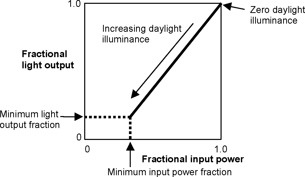
Figure 60. Control action for a continuous dimming
system.
Continuous/Off Dimming
Control[LINK]
A “continuous/off” dimming system has the same behavior as
a continuous dimming system except that the lights switch off
for fL < fL,min rather than
staying at fP,min.
Stepped Control[LINK]
For a stepped control system, fP takes
on discrete values depending on the range of
fLand the number of steps,
NL (Figure 61). This gives
\[{f_P} = \left\{
\begin{array}{l}0, & {\rm{if }}{f_L} =
0\\\frac{{{\mathop{\rm int}} ({N_L}{f_L}) + 1}}{{{N_L}}},
& {\rm{for }}0 < {f_L} < 1\\1, & {\rm{if
}}{f_L} = 1\end{array} \right.\]
If a lighting control probability,* pL, is
specified, fP* is set one level higher a
fraction of the time equal to 1-pL.
Specifically, if* fP* <1,*
fPà fP+
1/NL* if a random number between 0 and 1
exceeds pL. This can be used to simulate
the uncertainty associated with manual switching of
lights.
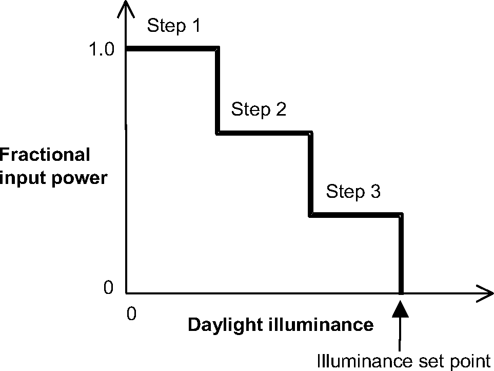
Figure 61. Stepped lighting control with three steps.
Lighting Power
Reduction[LINK]
Using the value of fPat each reference
point and the fraction fZ of the zone
controlled by the reference point, the net lighting power
multiplier, MP, for the entire zone is
calculated; this value multiplies the lighting power output
without daylighting.
\[{M_P} = \sum\limits_{{i_L} =
1}^2 {{f_P}({i_L})} {f_Z}({i_L}) + \left( {1 -
\sum\limits_{{i_L} = 1}^2 {} {f_Z}({i_L})}
\right)\]
In this expression, the term to the right in the
parentheses corresponds to the fraction of the zone not
controlled by either reference point. For this fraction the
electric lighting is unaffected and the power multiplier is
1.0.
CIE Technical Committee 4.2. 1973. Standardization of the
Luminance Distribution on Clear Skies. CIE Pub. No. 22,
Commission Internationale d’Eclairage, Paris.
Hopkinson, R.G., J. Longmore and P. Petherbridge. 1954. An
Empirical Formula for the Computation of the Indirect
Component of Daylight Factors. Trans. Illum. Eng. Soc.
(London) 19, 201.
Hopkinson, R.G., P. Petherbridge and J. Longmore. 1966.
Daylighting. Heinnemann, London, p. 322.
Hopkinson, R.G. 1970. Glare from Windows. Construction
Research and Development Journal 2, 98.
Hopkinson, R.G. 1972. Glare from Daylighting in Buildings.
Applied Ergonomics 3, 206.
Kittler, R. 1965. Standardization of Outdoor Conditions for
the Calculation of the Daylight Factor with Clear Skies. Proc.
CIE Inter-Session Meeting on Sunlight,
Newcastle-Upon-Tyne.
Lynes, J.A. 1968. Principles of Natural Lighting. Applied
Science Publishers, Ltd., London, p. 129.
Matsuura, K. 1987. Luminance Distributions of Various
Reference Skies. CIE Technical Report of TC 3-09.
Moon, P. and D. Spencer. 1942. Illumination from a
Nonuniform Sky. Illuminating Engineering 37, 707-726.
[1] For beam incident on an
exterior window we have the following: For transparent glass
with no shade or blind there is only beam-to-beam
transmission. For diffusing glass, or if a window shade is in
place, there is only beam-to-diffuse transmission. If a window
blind is in place there is beam-to-diffuse transmission, and,
depending on slat angle, solar profile angle, etc., there can
also be beam-to-beam transmission.
[2] See “Beam Solar Reflection from
Window
Reveal Surfaces.”
[3] If Solar Distribution =
FullInteriorAndExterior in the Building
object, the program calculates where beam solar from exterior
windows falls inside the zone. Otherwise, all beam solar is
assumed to fall on the floor.
[4] For the purposes of the surface
heat balance calculation, any beam solar radiation absorbed by
a surface is assumed to be uniformly distributed over the
surface even though in reality it is likely to be concentrated
in one or more discrete patches on the surface.
[5]
TBmiis zero if the window has
diffusing glass or a shade. TBmi can be
> 0 if a blind is present and the slat angle, solar profile
angle, etc., are such that some beam passes between the
slats.
[6] A different method from that
described here is used for calculating reflections from
daylighting shelves (see “Daylighting Shelves”).
[7] The ground surface is assumed
to be diffusely reflecting so there is no specular reflection
from the ground. The program could be improved by adding a
ground surface specular component, which could be important
for snow-cover conditions.
[8] The sun positions for which the
daylight factors are calculated are the same as those for
which the solar shadowing calculations are done.
Perez, R., P. Ineichen, R. Seals, J. Michalsky and R.
Stewart. 1990. Modeling Daylight Availability and Irradiance
Components from Direct and Global Irradiance. Solar Energy 44,
271-289.
Petherbridge, P. and J. Longmore. 1954. Solid Angles
Applied to Visual Comfort Problems. Light and Lighting
47,173.
Winkelmann, F.C. 1983. Daylighting Calculation in
DOE-2. Lawrence Berkeley Laboratory report no.
LBL-11353, January 1983.
Winkelmann, F.C. and S. Selkowitz. 1985. Daylighting
Simulation in the DOE-2 Building
Energy Analysis Program. Energy and Buildings 8,
271-286.

Time-Step Daylighting Calculation[LINK]
Overview[LINK]
A daylighting calculation is performed each time step that the sun is up for each zone that has one or two daylighting reference points specified. The exterior horizontal illuminance from the sun and sky is determined from solar irradiance data from the weather file. The interior illuminance at each reference point is found for each window by interpolating the daylight illuminance factors for the current sun position, then, for sky-related interior illuminance, multiplying by the exterior horizontal illuminance from the appropriate sky types that time step, and, for sun-related interior illuminance, multiplying by the exterior horizontal solar illuminance that time step. By summation, the net illuminance and glare due to all of the windows in a zone are found. If glare control has been specified window shading (by movable shading devices or switchable glazing) is deployed to reduce glare. Finally the illuminance at each reference point for the final window and shade configuration is used by the lighting control system simulation to determine the electric lighting power required to meet the illuminance setpoint at each reference point.
Table 27. Variables in Time-Step CalculationsTime-Step Sky Luminance[LINK]
The sky luminance distribution, ψ, for a particular time step is expressed as a linear interpolation of two of the four standard skies — ψcs, ψts , ψis and ψos — described above under “Sky Luminance Distributions.” The two sky types that are interpolated depend on the value of the sky clearness. The interpolation factors are a function of sky clearness and sky brightness (Perez et al., 1990). Sky clearness is given by
\[\varepsilon = \frac{{\frac{{{S_{h,dif}} + {S_{norm,dir}}}}{{{S_{h,dif}}}} + \kappa {Z^3}}}{{1 + \kappa {Z^3}}}\]
where Sh,dif is the diffuse horizontal solar irradiance, Snorm,diris the direct normal solar irradiance, Z is the solar zenith angle and κ is a constant equal to 1.041 for Z in radians.
Sky brightness is given by
\[\Delta = {S_{h,dif}}m/S_{norm,dir}^{ext}\]
where m is the relative optical air mass and \(S_{norm,dir}^{ext}\) is the extraterrestrial direct normal solar irradiance.
If ε ≤ 1.2
\[{\psi_{is,os}} = {s_{is,os}}{\psi_{is}} + (1 - {s_{is,os}}){\psi_{os}}\]
where ψis is the intermediate sky luminance distribution, ψos is the overcast sky luminance distribution, and
\[{s_{is,os}} = \min \{ 1,\max [0,(\varepsilon - 1)/0.2,(\Delta - 0.05)/0.4]\}\]
If 1.2<ε ≤ 3
\[{\psi_{ts,is}} = {s_{ts,is}}{\psi_{ts}} + (1 - {s_{ts,is}}){\psi_{is}}\]
where ψts is the clear turbid sky luminance distribution and
\[{s_{ts,is}} = (\varepsilon - 1.2)/1.8\]
If ε > 3
\[{\psi_{cs,ts}} = {s_{cs,ts}}{\psi_{cs}} + (1 - {s_{cs,ts}}){\psi_{ts}}\]
where ψcs is the clear sky luminance distribution and
\[{s_{cs,ts}} = \min [1,(\varepsilon - 3)/3]\]
Interior Illuminance[LINK]
For each time step the interior illuminance, Iwin, from a window is calculated as follows by multiplying daylight factors and exterior illuminance.
First, the sun- and sky-related daylight illuminance factors for the time step are determined by interpolation of the hourly factors:
\[{\bar d_{sun}}({i_L},{i_S}) = {w_j}{d_{sun}}({i_L},{i_S},{i_h}) + (1 - {w_j}){d_{sun}}({i_L},{i_S},{i_h} + 1)\]
\[{\bar d_{sky,k}}({i_L},{i_S}) = {w_j}{d_{sky,k}}({i_L},{i_S},{i_h}) + (1 - {w_j}){d_{sky,k}}({i_L},{i_S},{i_h} + 1)\]
where iL is the reference point index (1 or 2), iS is the window shade index (1 for unshaded window, 2 for shaded window),* ih* is the hour number, and k is the sky type index. For the* j*th time step in an hour, the time-step interpolation weight is given by
\[{w_j} = 1 - \min [1,j/{N_t}]\]
where Nt is the number of time steps per hour.
The interior illuminance from a window is calculated as
\[{I_{win}}({i_L},{i_S}) = {\bar d_{sun}}{E_{h,sun}} + [{\bar d_{sky,k}}({i_L},{i_S}){f_k} + {\bar d_{sky,k'}}({i_L},{i_S}){f_{k'}}]{E_{h,sky}}\]
where Eh,sun and Eh,sky are the exterior horizontal illuminance from the sun and sky, respectively, and fk and fk’ are the fraction of the exterior horizontal illuminance from the sky that is due to sky type k and k’, respectively.
The horizontal illuminance from sun and sky are given by
\[\begin{array}{rl} E_{h,sun} & = \eta_{dir} S_{norm,dir} \cos Z \\ E_{h,sky} & = \eta_{dif} S_{h,dif} \end{array}\]
where Z is the solar zenith angle, ηdif is the luminous efficacy (in lumens/Watt) of diffuse solar radiation from the sky and ηdir is the luminous efficacy of direct radiation from the sun. The efficacies are calculated from direct and global solar irradiance using a method described in (Perez et al, 1990).
The fractions fk and fk’ are given by
\[\begin{array}{rl} f_k & = \frac{ s_{k,k'} E_{h,k} } { s_{k,k'} E_{h,k} + (1 - s_{k,k'})E_{h,k'}} \\ f_{k'} & = \frac{ (1 - s_{k,k'} ) E_{h,k'} } { s_{k,k'} E_{h,k} + (1 - s_{k,k'} ) E_{h,k'}} \end{array}\]
where Eh,k and Eh,k’ are the horizontal illuminances from skies k and k’, respectively (see “Exterior Horizontal Luminance,” above), and sk,k’ is the interpolation factor for skies kand k’(see “Time-Step Sky Luminance,” above). For example, if ε > 3, k = cs (clear sky), k’ = ts (clear turbid sky) and
\(s_{k,k'} = s_{cs,ts} = \min [1,(\varepsilon - 3)/3]\)
Similarly, the window source luminance, Swin, and window background luminance, Bwin, for a window are calculated from
\[{S_{win}}({i_L},{i_S}) = {\bar w_{sun}}{E_{h,sun}} + [{\bar w_{sky,k}}({i_L},{i_S}){f_k} + {\bar w_{sky,k'}}({i_L},{i_S}){f_{k'}}]{E_{h,sky}}\]
\[{B_{win}}({i_L},{i_S}) = {\bar b_{sun}}{E_{h,sun}} + [{\bar b_{sky,k}}({i_L},{i_S}){f_k} + {\bar b_{sky,k'}}({i_L},{i_S}){f_{k'}}]{E_{h,sky}}\]
The total illuminance at a reference point from all of the exterior windows in a zone is
\[{I_{tot}}({i_L}) = \sum\limits_{\scriptstyle{\rm{windows}}\atop\scriptstyle{\rm{in zone}}} {{I_{win}}({i_s},{i_L})}\]
where* iS* = 1 if the window is unshaded and iS = 2 if the window is shaded that time step. (Before the illuminance calculation is done the window shading control will have been simulated to determine whether or not the window is shaded.)
Similarly, the total background luminance is calculated:
\[{B_{tot}}({i_L}) = \sum\limits_{\scriptstyle{\rm{windows}}\atop\scriptstyle{\rm{in zone}}} {{B_{win}}({i_s},{i_L})}\]
Glare Index[LINK]
The net glare index at each reference point is calculated as
\[{G_I}({i_L}) = 10{\log_{10}}\sum\limits_{\scriptstyle{\rm{windows}}\atop\scriptstyle{\rm{in zone}}} {\frac{{{S_{win}}{{({i_L},{i_S})}^{1.6}}\Omega {{({i_L})}^{0.8}}}}{{B({i_L}) + 0.07\omega {{({i_L})}^{0.5}}{S_{win}}({i_L},{i_S})}}}\]
where
\[B\left( {{i_L}} \right) = max\left( {{B_{win}}\left( {{i_L}} \right),{\rho_b}{I_{set}}\left( {{i_L}} \right)} \right)\]
In the last relationship, the background luminance is approximated as the larger of the background luminance from daylight and the average background luminance that would be produced by the electric lighting at full power if the illuminance on the room surfaces were equal to the setpoint illuminance. In a more detailed calculation, where the luminance of each room surface is separately determined, B(iL) would be better approximated as an area-weighted luminance of the surfaces surrounding a window, taking into account the luminance contribution from the electric lights.
Glare Control Logic[LINK]
If glare control has been specified and the glare index at either reference point exceeds a user-specified maximum value, GI,max, then the windows in the zone are shaded one by one in attempt to bring the glare at both points below GI,max. (Each time a window is shaded the glare and illuminance at each reference point is recalculated.) The following logic is used:
5) If there is only one reference point, shade a window if it is unshaded and shading it decreases the glare, even if it does not decrease the glare below GI,max. Note that if a window has already been shaded, say to control solar gain, it will be left in the shaded state.
6) If there are two reference points, then:
* If glare is too high at both points, shade the window if it decreases glare at both points.
If glare is too high only at the first point, shade the window if the glare at the first point decreases, and the glare at the second point stays belowGI,max*.
7) Shades are closed in the order of window input until glare at both points is below GI,max, or until there are no more windows left to shade.
Lighting Control System Simulation[LINK]
Once the final daylight illuminance value at each reference point has been determined, the electric lighting control is simulated. The fractional electric lighting output, fL, required to meet the setpoint at reference point iL is given by
\[{f_L}({i_L}) = {\rm{max}}\left[ {0,\frac{{{I_{set}}({i_L}) - {I_{tot}}({i_L})}}{{{I_{set}}({i_L})}}} \right]\]
Here, Iset is the illuminance setpoint and Itot is the daylight illuminance at the reference point. This relationship assumes that the electric lights at full power produce an illuminance equal to Iset at the reference point.
The fractional electric lighting input power, fP, corresponding to fL is then calculated. The relationship between fP and fL depends on the lighting control type.
Continuous Dimming Control[LINK]
For a continuously-dimmable control system, it is assumed that fP is constant and equal to fP,minfor fL<fL,min and that fP increases linearly from fP,min to 1.0 as fL increases from fL,min to 1.0 (Figure 60). This gives
\[{f_P} = \left\{ \begin{array}{l}{f_{P,\min }} & {\rm{for }}{f_L} < {f_{L,\min }}\\\frac{{{f_L} + (1 - {f_L}){f_{P,\min }} - {f_{L,\min }}}}{{1 - {f_{L,\min }}}}\end{array} \right.{\rm{ for }}{f_{L,\min }} \le {f_L} \le 1\]
Figure 60. Control action for a continuous dimming system.
Continuous/Off Dimming Control[LINK]
A “continuous/off” dimming system has the same behavior as a continuous dimming system except that the lights switch off for fL < fL,min rather than staying at fP,min.
Stepped Control[LINK]
For a stepped control system, fP takes on discrete values depending on the range of fLand the number of steps, NL (Figure 61). This gives
\[{f_P} = \left\{ \begin{array}{l}0, & {\rm{if }}{f_L} = 0\\\frac{{{\mathop{\rm int}} ({N_L}{f_L}) + 1}}{{{N_L}}}, & {\rm{for }}0 < {f_L} < 1\\1, & {\rm{if }}{f_L} = 1\end{array} \right.\]
If a lighting control probability,* pL, is specified, fP* is set one level higher a fraction of the time equal to 1-pL. Specifically, if* fP* <1,* fPà fP+ 1/NL* if a random number between 0 and 1 exceeds pL. This can be used to simulate the uncertainty associated with manual switching of lights.
Figure 61. Stepped lighting control with three steps.
Lighting Power Reduction[LINK]
Using the value of fPat each reference point and the fraction fZ of the zone controlled by the reference point, the net lighting power multiplier, MP, for the entire zone is calculated; this value multiplies the lighting power output without daylighting.
\[{M_P} = \sum\limits_{{i_L} = 1}^2 {{f_P}({i_L})} {f_Z}({i_L}) + \left( {1 - \sum\limits_{{i_L} = 1}^2 {} {f_Z}({i_L})} \right)\]
In this expression, the term to the right in the parentheses corresponds to the fraction of the zone not controlled by either reference point. For this fraction the electric lighting is unaffected and the power multiplier is 1.0.
References[LINK]
CIE Technical Committee 4.2. 1973. Standardization of the Luminance Distribution on Clear Skies. CIE Pub. No. 22, Commission Internationale d’Eclairage, Paris.
Hopkinson, R.G., J. Longmore and P. Petherbridge. 1954. An Empirical Formula for the Computation of the Indirect Component of Daylight Factors. Trans. Illum. Eng. Soc. (London) 19, 201.
Hopkinson, R.G., P. Petherbridge and J. Longmore. 1966. Daylighting. Heinnemann, London, p. 322.
Hopkinson, R.G. 1970. Glare from Windows. Construction Research and Development Journal 2, 98.
Hopkinson, R.G. 1972. Glare from Daylighting in Buildings. Applied Ergonomics 3, 206.
Kittler, R. 1965. Standardization of Outdoor Conditions for the Calculation of the Daylight Factor with Clear Skies. Proc. CIE Inter-Session Meeting on Sunlight, Newcastle-Upon-Tyne.
Lynes, J.A. 1968. Principles of Natural Lighting. Applied Science Publishers, Ltd., London, p. 129.
Matsuura, K. 1987. Luminance Distributions of Various Reference Skies. CIE Technical Report of TC 3-09.
Moon, P. and D. Spencer. 1942. Illumination from a Nonuniform Sky. Illuminating Engineering 37, 707-726.
[1] For beam incident on an exterior window we have the following: For transparent glass with no shade or blind there is only beam-to-beam transmission. For diffusing glass, or if a window shade is in place, there is only beam-to-diffuse transmission. If a window blind is in place there is beam-to-diffuse transmission, and, depending on slat angle, solar profile angle, etc., there can also be beam-to-beam transmission.
[2] See “Beam Solar Reflection from Window Reveal Surfaces.”
[3] If Solar Distribution = FullInteriorAndExterior in the Building object, the program calculates where beam solar from exterior windows falls inside the zone. Otherwise, all beam solar is assumed to fall on the floor.
[4] For the purposes of the surface heat balance calculation, any beam solar radiation absorbed by a surface is assumed to be uniformly distributed over the surface even though in reality it is likely to be concentrated in one or more discrete patches on the surface.
[5] TBmiis zero if the window has diffusing glass or a shade. TBmi can be > 0 if a blind is present and the slat angle, solar profile angle, etc., are such that some beam passes between the slats.
[6] A different method from that described here is used for calculating reflections from daylighting shelves (see “Daylighting Shelves”).
[7] The ground surface is assumed to be diffusely reflecting so there is no specular reflection from the ground. The program could be improved by adding a ground surface specular component, which could be important for snow-cover conditions.
[8] The sun positions for which the daylight factors are calculated are the same as those for which the solar shadowing calculations are done.
Perez, R., P. Ineichen, R. Seals, J. Michalsky and R. Stewart. 1990. Modeling Daylight Availability and Irradiance Components from Direct and Global Irradiance. Solar Energy 44, 271-289.
Petherbridge, P. and J. Longmore. 1954. Solid Angles Applied to Visual Comfort Problems. Light and Lighting 47,173.
Winkelmann, F.C. 1983. Daylighting Calculation in DOE-2. Lawrence Berkeley Laboratory report no. LBL-11353, January 1983.
Winkelmann, F.C. and S. Selkowitz. 1985. Daylighting Simulation in the DOE-2 Building Energy Analysis Program. Energy and Buildings 8, 271-286.
Documentation content copyright © 1996-2026 The Board of Trustees of the University of Illinois and the Regents of the University of California through the Ernest Orlando Lawrence Berkeley National Laboratory. All rights reserved. EnergyPlus is a trademark of the US Department of Energy.
This documentation is made available under the EnergyPlus Open Source License v1.0.