Internal Cumbustion
Engine[LINK]
The engine-driven generator model was originally developed
for the BLAST program and was subsequently adapted for use in
EnergyPlus. The model uses the following set of equations all
of which are quadratic fits to the PLR (Part Load Ratio) of
the generator. The coefficients must be derived from
manufacturers data.
The electrical load and engine generator nominal load
capacity are used to compute the part load ratio.
The exhaust gas temp and flow rate are used if a stack heat
exchanger is used to recover waste heat from the exhaust. This
temperature is the inlet temperature to the heat exchanger
which is modeled in a UA-effectiveness form:
The exhaust flow rate is then calculated as:
where Treference is the reference temperature
for the fuel lower heating value, and is given as 25°C in
manufacturer’s data, and
Finally heat recovered from the lube oil and the water
jacket are accounted for as follows:
The manufacturer must supply the recoverable water jacket
heat, lube oil heat and exhaust heat and associated fuel
consumption for a range of load conditions. This data is then
fit to the PLR to obtain the fifteen a,b,c,d, and e
coefficients.
Turbine Generator[LINK]
The combustion turbine generator model was originally
developed for the BLAST program and was subsequently adapted
for use in EnergyPlus. The model uses the following set of
equations all of which are equation fits to the PLR (Part Load
Ratio) of the generator and the entering air temperature. The
coefficients must be derived from manufacturers data. For
electric power generated in Watts, the fuel input rate is
calculated in J/s.
The electrical load and engine generator nominal load
capacity are used to compute the part load ratio.
The temperature difference shows the deviation of ambient
air temperature from the manufacturers design air
temperature.
A second curve fit calculates the exhaust temperature (C)
by multiplying the exhaust temperature (C) for a particular
part load by a correction factor based on the deviation from
design temperature.
The exhaust gas temp is used if a stack heat exchanger is
used to recover waste heat from the exhaust. This temperature
is the inlet temperature to the heat exchanger which is
modeled in a UA-effectiveness form:
Where the design minimum exhaust temperature is a user
input to the model and the exhaust mass flow rate and the UA
are fit from manufacturers data as follows:
Finally, heat recovered from the lube oil is accounted for
as follows:
Microturbine Generator[LINK]
Microturbine generators are small combustion turbines that
produce electricity on a relatively small scale (e.g., 25kW to
500kW). This model uses nominal performance at reference
conditions along with several modifier curves to determine
electrical power output and fuel use at non-reference
conditions. The modifier curve coefficients must be derived
from manufacturers data. Standby and ancillary power can also
be taken into account.
Exhaust air energy recovery for heating water can be also
be modeled. Similar to electrical power output, thermal power
(heat recovery to water) output is calculated using nominal
performance at reference conditions with modifier curves to
account for variations at non-reference conditions. The ElectricLoadCenter:Generators
and ElectricLoadCenter:Distribution
objects are used to define the availability and control of the
electric generators included in the simulation (ref. ElectricLoadCenter:Generators
and ElectricLoadCenter:Distribution).
For each simulation time step that the generator is being
asked to operate (i.e., produce electrical power as determined
by the ElectricLoadCenter), the full load electrical output of
the generator is determined using the user-defined reference
electrical power output along with a bi-quadratic modifier
curve to account for differences in the combustion air inlet
temperature and elevation for the current simulation time step
compared to the reference temperature and elevation (i.e., the
modifier curve should evaluate to 1.0 at the reference
combustion air inlet temperature and reference elevation).
where:
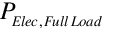 = Full load electrical
power output (W)
= Full load electrical
power output (W)
 = Reference Electrical
Power Output, user input (W)
= Reference Electrical
Power Output, user input (W)
 = User-defined Electric
Power Modifier Curve (function of temperature and elevation)
evaluated at the current combustion air inlet temperature and
elevation
= User-defined Electric
Power Modifier Curve (function of temperature and elevation)
evaluated at the current combustion air inlet temperature and
elevation
 = Combustion air inlet
temperature (°C)
= Combustion air inlet
temperature (°C)
 = Elevation (m). This
value obtained from the Location object or the weather
file.
= Elevation (m). This
value obtained from the Location object or the weather
file.
The full load electrical power output of the generator is
then checked against the minimum and maximum full load
electrical power outputs specified by the user:
 = Maximum Full Load
Electrical Power Output, user input (W)
= Maximum Full Load
Electrical Power Output, user input (W)
 = Minimum Full Load
Electrical Power Output, user input (W)
= Minimum Full Load
Electrical Power Output, user input (W)
The actual (operating) electrical power output from the
generator is determined next based on the load requested by
the Electric Load Center, the generator’s minimum and maximum
part-load ratios, and the ancillary power.
where:
 = Actual (operating)
electrical power output (W)
= Actual (operating)
electrical power output (W)
 = Electrical power output
being requested by the Electric Load Center (W)
= Electrical power output
being requested by the Electric Load Center (W)
 = Ancillary Power, user
input (W)
= Ancillary Power, user
input (W)
 = Part-load ratio of the
electric generator
= Part-load ratio of the
electric generator
 = Maximum part-load ratio
of the electric generator (i.e., the maximum value for the
independent variable [PLR] defined in the Curve:Quadratic
or Curve:Cubic
object for the Electrical Efficiency Modifier Curve [function
of part-load ratio])
= Maximum part-load ratio
of the electric generator (i.e., the maximum value for the
independent variable [PLR] defined in the Curve:Quadratic
or Curve:Cubic
object for the Electrical Efficiency Modifier Curve [function
of part-load ratio])
 = Minimum part-load ratio
of the electric generator (i.e., the minimum value for the
independent variable [PLR] defined in the Curve:Quadratic
or Curve:Cubic
object for the Electrical Efficiency Modifier Curve [function
of part-load ratio])
= Minimum part-load ratio
of the electric generator (i.e., the minimum value for the
independent variable [PLR] defined in the Curve:Quadratic
or Curve:Cubic
object for the Electrical Efficiency Modifier Curve [function
of part-load ratio])
The generator’s electrical efficiency is then calculated
based on the user-specified reference electrical efficiency
(lower heating value [LHV] basis) and two electrical
efficiency modifier curves.
where:
 = User-defined Electrical
Efficiency Modifier Curve (function of temperature) evaluated
at the current combustion air inlet temperature
= User-defined Electrical
Efficiency Modifier Curve (function of temperature) evaluated
at the current combustion air inlet temperature
 = User-defined Electrical
Efficiency Modifier Curve (function of part-load ratio)
evaluated at the current operating part-load ratio
= User-defined Electrical
Efficiency Modifier Curve (function of part-load ratio)
evaluated at the current operating part-load ratio
 = Electrical efficiency
at the current operating conditions
= Electrical efficiency
at the current operating conditions
 = Reference Electrical
Efficiency (LHV [lower heating value] Basis), user input
= Reference Electrical
Efficiency (LHV [lower heating value] Basis), user input
The fuel energy consumption rate (LHV Basis) is then
calculated as follows:
where:
 = Fuel energy consumption
rate, LHV basis (W)
= Fuel energy consumption
rate, LHV basis (W)
If ElecEffOperating is equal to zero,
then POperating and  ~~are set to zero. The fuel mass
flow rate is then calculated.
~~are set to zero. The fuel mass
flow rate is then calculated.
where:
 = Mass flow rate of fuel
being consumed by the generator (kg/s), report variable
“Generator Mass Flow Rate [kg/s]”
= Mass flow rate of fuel
being consumed by the generator (kg/s), report variable
“Generator Mass Flow Rate [kg/s]”
LHV = Fuel Lower Heating Value, user input
(kJ/kg)
The ancillary power is calculated next using the
user-specified ancillary power and ancillary power modifier
curve. The ancillary power modifier curve is a quadratic
function with the generator’s fuel mass flow rate as the
independent variable. If an ancillary power modifier curve is
not specified in the input file, the modifier is assumed to be
1.0 and the ancillary power will be constant throughout the
simulation.
where:
 = User-defined Ancillary
Power Modifier Curve (function of fuel input) evaluated at the
actual fuel mass flow rate. This multiplier is assumed to be
1.0 if an ancillary power modifier curve name is not specified
in the input.
= User-defined Ancillary
Power Modifier Curve (function of fuel input) evaluated at the
actual fuel mass flow rate. This multiplier is assumed to be
1.0 if an ancillary power modifier curve name is not specified
in the input.
 = Ancillary power, user
input (W)
= Ancillary power, user
input (W)
 = Ancillary electric
power at the current fuel mass flow rate (W), report variable
“Generator Ancillary Electric Power [W]”.
= Ancillary electric
power at the current fuel mass flow rate (W), report variable
“Generator Ancillary Electric Power [W]”.
If ancillary power is constant for the simulation (e.g., no
modifier curve defined), then the calculations continue as
described below. However, if an ancillary power modifier curve
has been defined, then the calculations described above for
PElecOperating,
ElecEffOperating,  ~~and
PAncillary,Operating are recalculated in
sequence until the solution converges.
~~and
PAncillary,Operating are recalculated in
sequence until the solution converges.
The generator’s “net” electrical power output is calculated
as the difference between the generator’s actual power output
and the ancillary electric power as follows.
where:
 = Generator net electric
power output, report variable “Generator Produced Electric
Power [W]”
= Generator net electric
power output, report variable “Generator Produced Electric
Power [W]”
The fuel energy consumption rate (higher heating value
basis) for the generator is then calculated as follows:
where:
 = fuel energy consumption
rate (W), report variables “Generator HHV Basis Rate [W]” and
“Generator Fuel HHV Basis Rate [W]”
= fuel energy consumption
rate (W), report variables “Generator HHV Basis Rate [W]” and
“Generator Fuel HHV Basis Rate [W]”
 = Fuel Higher Heating
Value, user input (kJ/kg)
= Fuel Higher Heating
Value, user input (kJ/kg)
Standby electrical power may also be modeled to simulate
controls or other parasitics used by the generator. The
standby power is calculated only when the generator is not
operating (i.e., Load from the Electric Load Center
is zero). If the generator operates for a given timestep
(i.e., Load > 0.0), the standby power is set equal
to 0.
where:
 = Standby power, user
input (W)
= Standby power, user
input (W)
 = Report variable
“Generator Standby Electric Power” (W)
= Report variable
“Generator Standby Electric Power” (W)
Report variables for electric energy produced, electric
efficiency (LHV basis), fuel consumption (HHV basis), standby
electric consumption and ancillary electric consumption are
calculated as follows:
where:
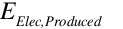 = Report variable
“Generator Produced Electric Energy [J]”
= Report variable
“Generator Produced Electric Energy [J]”
 = Report variable
“Generator LHV Basis Electric Efficiency [-]”
= Report variable
“Generator LHV Basis Electric Efficiency [-]”
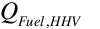 = Report variables
“Generator HHV Basis Energy [J]” and “Generator Fuel HHV Basis
Energy [J]”
= Report variables
“Generator HHV Basis Energy [J]” and “Generator Fuel HHV Basis
Energy [J]”
 = Report variable
“Generator Standby Electric Energy [J]”
= Report variable
“Generator Standby Electric Energy [J]”
 = Report variable
“Generator Ancillary Electric Energy [J]”
= Report variable
“Generator Ancillary Electric Energy [J]”
TimeStepSys = HVAC system simulation time step
(hr)
In addition to calculating electric power production and
fuel usage, the model is able to determine thermal power (heat
recovery) output for heating water. For this case, the water
flow rate through the heat recovery heat exchanger is
established first. If the Heat Recovery Water Flow Operating
Mode (user input) is set to Plant Control, then the Reference
Heat Recovery Water Flow Rate (user input) is requested
whenever the generator operates (constant value), but the
actual flow rate may be restricted by other plant components
(e.g., pump). If the Heat Recovery Water Flow Operating Mode
is set to Internal Control, then the requested water flow when
the generator operates is determined by the Reference Heat
Recovery Water Flow Rate and a flow rate modifier curve.
where:
 = Report variable
“Generator Heat Recovery Water Mass Flow Rate [kg/s]”
= Report variable
“Generator Heat Recovery Water Mass Flow Rate [kg/s]”
 = Reference Heat Recovery
Water Flow Rate (m3/s), user input
= Reference Heat Recovery
Water Flow Rate (m3/s), user input
 = Density of water
(kg/m3) at 5.05°C
= Density of water
(kg/m3) at 5.05°C
 = User-defined Heat
Recovery Water Flow Rate Modifier Curve (function of
temperature and power) evaluated at the current inlet water
temperature and net electrical power output. This multiplier
is assumed to be 1.0 if a water flow rate modifier curve name
is not specified in the input.
= User-defined Heat
Recovery Water Flow Rate Modifier Curve (function of
temperature and power) evaluated at the current inlet water
temperature and net electrical power output. This multiplier
is assumed to be 1.0 if a water flow rate modifier curve name
is not specified in the input.
 = Heat recovery inlet
water temperature (°C), report variable “Generator Heat
Recovery Inlet Temperature [C]”
= Heat recovery inlet
water temperature (°C), report variable “Generator Heat
Recovery Inlet Temperature [C]”
 = Net electrical power
output from the generator (W)
= Net electrical power
output from the generator (W)
The methodology for determining thermal power (heat
recovery to water) is similar to that used for calculating
electric power production. The generator’s steady-state
thermal efficiency is calculated based on the user-specified
reference thermal efficiency (LHV basis) and a thermal
efficiency modifier curve.
where:
 = Steady-state thermal
efficiency at current conditions
= Steady-state thermal
efficiency at current conditions
 = Reference Thermal
Efficiency (LHV Basis), user input
= Reference Thermal
Efficiency (LHV Basis), user input
 = User-defined Thermal
Efficiency Modifier Curve (function of temperature and
elevation) evaluated at the current combustion air inlet
temperature and elevation. This multiplier is assumed to be
1.0 if a thermal efficiency modifier curve name is not
specified in the input.
= User-defined Thermal
Efficiency Modifier Curve (function of temperature and
elevation) evaluated at the current combustion air inlet
temperature and elevation. This multiplier is assumed to be
1.0 if a thermal efficiency modifier curve name is not
specified in the input.
The steady-state thermal power produced (heat recovery
rate) is then calculated:
The actual (operating) thermal power is then calculated
using the steady-state thermal power and three modifier
curves:


where:
 = Report variable
“Generator Produced Thermal Rate [W]”
= Report variable
“Generator Produced Thermal Rate [W]”
 = User-defined Heat
Recovery Rate Modifier Curve (function of part-load ratio)
evaluated at the current operating part-load ratio. This
multiplier is assumed to be 1.0 if a modifier curve name is
not specified in the input.
= User-defined Heat
Recovery Rate Modifier Curve (function of part-load ratio)
evaluated at the current operating part-load ratio. This
multiplier is assumed to be 1.0 if a modifier curve name is
not specified in the input.
 = User-defined Heat
Recovery Rate Modifier Curve (function of inlet water
temperature) evaluated at the current inlet water temperature.
This multiplier is assumed to be 1.0 if a modifier curve name
is not specified in the input.
= User-defined Heat
Recovery Rate Modifier Curve (function of inlet water
temperature) evaluated at the current inlet water temperature.
This multiplier is assumed to be 1.0 if a modifier curve name
is not specified in the input.
 = User-defined Heat
Recovery Rate Modifier Curve (function of water flow rate)
evaluated at the current heat recovery water flow rate. This
multiplier is assumed to be 1.0 if a modifier curve name is
not specified in the input.
= User-defined Heat
Recovery Rate Modifier Curve (function of water flow rate)
evaluated at the current heat recovery water flow rate. This
multiplier is assumed to be 1.0 if a modifier curve name is
not specified in the input.
The heat recovery output water temperature is then
calculated.
where:
 = Heat recovery outlet
water temperature (°C), report variable “Generator Heat
Recovery Outlet Temperature [C]”
= Heat recovery outlet
water temperature (°C), report variable “Generator Heat
Recovery Outlet Temperature [C]”
 = Heat capacity of water
(J/kg-K)
= Heat capacity of water
(J/kg-K)
If the calculated heat recovery outlet water temperature
exceeds to Maximum Heat Recovery Water Temperature (user
input), then the outlet water temperature is reset to the
maximum temperature (user input) and the thermal power is
recalculated.
If combustion air inlet and outlet node names are specified
in the input, along with exhaust air flow rate and exhaust air
temperature information, then the model calculates the exhaust
air conditions for each simulation time step. The exhaust air
mass flow rate is first calculated based on the Reference
Exhaust Air Mass Flow Rate, two modifier curves and an air
density adjustment. Since fans are volumetric flow devices,
the ratio of the air density at actual inlet air conditions to
air density at reference inlet air conditions is used as an
adjustment factor.


where:
 = Exhaust air mass flow
rate (kg/s)
= Exhaust air mass flow
rate (kg/s)
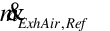 = Reference Exhaust Air
Mass Flow Rate (kg/s), user input
= Reference Exhaust Air
Mass Flow Rate (kg/s), user input
 = User-defined Exhaust
Air Flow Rate Modifier Curve (function of temperature)
evaluated at the current combustion air inlet temperature.
This multiplier is assumed to be 1.0 if a modifier curve name
is not specified in the input.
= User-defined Exhaust
Air Flow Rate Modifier Curve (function of temperature)
evaluated at the current combustion air inlet temperature.
This multiplier is assumed to be 1.0 if a modifier curve name
is not specified in the input.
 = User-defined Exhaust
Air Flow Rate Rate Modifier Curve (function of part-load
ratio) evaluated at the current operating part-load ratio.
This multiplier is assumed to be 1.0 if a modifier curve name
is not specified in the input.
= User-defined Exhaust
Air Flow Rate Rate Modifier Curve (function of part-load
ratio) evaluated at the current operating part-load ratio.
This multiplier is assumed to be 1.0 if a modifier curve name
is not specified in the input.
 = Density of the
combustion inlet air (kg/m3)
= Density of the
combustion inlet air (kg/m3)
 = Density of combustion
inlet air at reference conditions (kg/m3)
= Density of combustion
inlet air at reference conditions (kg/m3)
In an analogous fashion, the exhaust air temperature is
calculated using the Nominal (reference) Exhaust Air Outlet
Temperature and two modifier curves.


where:
 = Exhaust air outlet
temperature (°C)
= Exhaust air outlet
temperature (°C)
 = Nominal Exhaust Air
Outlet Temperature (°C), user input
= Nominal Exhaust Air
Outlet Temperature (°C), user input
 = User-defined Exhaust
Air Temperature Modifier Curve (function of temperature)
evaluated at the current combustion air inlet temperature.
This multiplier is assumed to be 1.0 if a modifier curve name
is not specified in the input.
= User-defined Exhaust
Air Temperature Modifier Curve (function of temperature)
evaluated at the current combustion air inlet temperature.
This multiplier is assumed to be 1.0 if a modifier curve name
is not specified in the input.
 = User-defined Exhaust
Air Flow Rate Rate Modifier Curve (function of part-load
ratio) evaluated at the current operating part-load ratio.
This multiplier is assumed to be 1.0 if a modifier curve name
is not specified in the input.
= User-defined Exhaust
Air Flow Rate Rate Modifier Curve (function of part-load
ratio) evaluated at the current operating part-load ratio.
This multiplier is assumed to be 1.0 if a modifier curve name
is not specified in the input.
The above calculations for exhaust air outlet temperature
assume no heat recovery to water is being done. If thermal
power (water heating) is being produced, then the exhaust air
outlet temperature is recalculated as follows:
where:
 = Heat capacity of air at
the actual combustion air inlet conditions (J/kg-K)
= Heat capacity of air at
the actual combustion air inlet conditions (J/kg-K)
The exhaust air outlet humidity ratio is also
calculated.
where:
 = Exhaust air outlet
humidity ratio (kg/kg)
= Exhaust air outlet
humidity ratio (kg/kg)
 = Exhaust air inlet
humidity ratio (kg/kg)
= Exhaust air inlet
humidity ratio (kg/kg)
 = Enthalpy of
vaporization of moisture at 16°C (J/kg)
= Enthalpy of
vaporization of moisture at 16°C (J/kg)
The remaining report variables are calculated as
follows.
where:
 = Report variable
“Generator Produced Thermal Energy [J]”
= Report variable
“Generator Produced Thermal Energy [J]”
 = Report variable
“Generator Thermal Efficiency LHV Basis [-]”
= Report variable
“Generator Thermal Efficiency LHV Basis [-]”
Micro-Cogenerator[LINK]
The input object Generator:MicroCHP
provides a model that is a direct implementation of a model
developed by IEA Annex 42 – The Simulation of
Building-Integrated Fuel Cell and Other Cogeneration Systems
(FC+COGEN-SIM). Annex 42 was formed as a working group within
the International Energy Agency (IEA) program on Energy
Conservation in Buildings and Community Systems (ECBCS). A
full description of the model specification can be found in
the report by Subtask B of FC+COGEN-SIM with the title
“Specifications for Modelling Fuel Cell and Combustion-Based
Residential Cogeneration Device within Whole-Building
Simulation Programs.” The “Micro CHP” model in EnergyPlus is
the one referred to as “A Generic Model for Combustion-based
Residential Cogeneration Devices.”
The Micro CHP model is a straightforward empirical model
with the exception that it is dynamic with respect to thermal
heat recovery where performance is cast as a function of
engine temperature. It is also dynamic with respect to
possible warm up and cool down periods that may affect the
ability of the generator to deliver the requested power. The
relevant model equations are:
where,
 is the steady-state, part
load, electrical conversion efficiency of the engine (-)
is the steady-state, part
load, electrical conversion efficiency of the engine (-)
 is the steady-state part
load, thermal conversion efficiency of the engine (-)
is the steady-state part
load, thermal conversion efficiency of the engine (-)
 is the mass flow rate of
plant fluid through the heat recovery section [kg/s]
is the mass flow rate of
plant fluid through the heat recovery section [kg/s]
 is the bulk temperature
of the plant fluid entering the heat recovery section
(oC)
is the bulk temperature
of the plant fluid entering the heat recovery section
(oC)
 is the bulk temperature
of the plant fluid leaving the heat recovery section
(oC)
is the bulk temperature
of the plant fluid leaving the heat recovery section
(oC)
 is the steady-state
electrical output of the system (W),
is the steady-state
electrical output of the system (W),
 is the gross heat input
into the engine (W),
is the gross heat input
into the engine (W),
 is the steady-state rate
of heat generation within the engine (W)
is the steady-state rate
of heat generation within the engine (W)
 is the lower heating
value of the fuel used by the system (J/kg or J/kmol),
is the lower heating
value of the fuel used by the system (J/kg or J/kmol),
 is the molar fuel flow
rate (kmol/s)
is the molar fuel flow
rate (kmol/s)
 is the mass fuel flow
rate (kg/s)
is the mass fuel flow
rate (kg/s)
 is the mass flow rate of
air thru the engine (kg/s)
is the mass flow rate of
air thru the engine (kg/s)
 is the thermal
capacitance of the engine control volume (W/K)
is the thermal
capacitance of the engine control volume (W/K)
 is the temperature of the
engine control volume (C)
is the temperature of the
engine control volume (C)
 is the effective thermal
conductance between the engine control volume and the cooling
water control volume (W/K).
is the effective thermal
conductance between the engine control volume and the cooling
water control volume (W/K).
 is the effective thermal
conductance between the engine control volume and the
surrounding environment (W/K)
is the effective thermal
conductance between the engine control volume and the
surrounding environment (W/K)
 is the air temperature of
the surrounding environment (C)
is the air temperature of
the surrounding environment (C)
 is the thermal
capacitance of the encapsulated cooling water and heat
exchanger shell in immediate thermal contact (J/K)
is the thermal
capacitance of the encapsulated cooling water and heat
exchanger shell in immediate thermal contact (J/K)
 is the thermal capacity
flow rate associated with the cooling water (W/K)
is the thermal capacity
flow rate associated with the cooling water (W/K)
The functional forms for  and
and  are 2nd order
trivariate polynomials with all of the cross terms.
are 2nd order
trivariate polynomials with all of the cross terms.
EnergyPlus solves these for state values for the engine
mass temperature,  , and the
outlet plant node,
, and the
outlet plant node,  , in the
following manner. The last two equations are interrelated but
otherwise ordinary differential equations with the general
form
, in the
following manner. The last two equations are interrelated but
otherwise ordinary differential equations with the general
form
and have analytical solution
The engine temperature at the current timestep is
calculated using
The plant node outlet fluid temperature (heat recovered) is
solved using
The interrelation of these two is handled by sequential
substitution using an iteration scheme that alternates between
calculations of  and
and  . The iteration loop exits once
the energy is determined to be balanced using the following
criteria:
. The iteration loop exits once
the energy is determined to be balanced using the following
criteria:
Number of iterations > 3\


The Micro CHP model has a number of different operating
modes. The operating mode for a given system timestep is
determined from the mode during the previous timestep, user
inputs, and high-level controls from elsewhere in EnergyPlus.
The operating mode is reported for the state at the end of
each timestep. The following table summarizes the various
operating modes and the criteria for switching to a new mode
for any given timestep. The EnergyPlus implementation adds the
“Off” mode to the modes specified by Annex 42 which
corresponds to the unit being scheduled to be unavailable. The
difference between OFF and Standby modes determines whether or
not standby power is consumed.
| Operating
mode |
Main
Criteria |
Notes |
| Off |
Availability schedule value =
0 |
No consumption of power or
fuel. |
| Stand By |
Availability schedule value ≠
0 |
Consumes stand by power but no
fuel |
| Warm Up |
Load (thermal or electric) >
0.0 |
Availability schedule value ≠
0 |
| Normal Operation |
Load (thermal or electric) >
0.0Availability schedule value ≠ 0Time Delay > elapsed time
since entering warm up mode |
Engine temp >= nominal
temp |
| Cool Down |
Load (thermal or electric) =
0.0 |
Availability schedule value ≠
0 |
For timesteps where the generator switches from warm up
mode to normal mode in the middle of the timestep, part load
ration values are calculated for the portion of the time step
that the generator is in normal operation.
The engine and heat recovery thermal conditions are modeled
for all modes so, for example, an engine that is off but still
warm could provide some hot water recovery.
The engine model can use an arbitray fuel mixture that is
defined by the user – see the entry for Generator:FuelSupply.
Kelly, N. and A. Ferguson. 2007. A Generic Model
Specification for Combustion-based Residential Cogeneration
Devices. In Specifications for Modelling Fuel Cell and
Combustion-Based Residential Cogeneration Device within
Whole-Building Simulation Programs. I.
Beausoleil-Morrison and N. Kelly editors. Draft report of
Annex 42 of the International Energy Agency ECBCS.
Fuel Cell Cogenerator[LINK]
The Generator:FuelCell
input objects provides a model which is a direct
implementation of a model developed by IEA Annex 42 – The
Simulation of Building-Integrated Fuel Cell and Other
Cogeneration Systems (FC+COGEN-SIM). Annex 42 was formed as a
working group within the International Energy Agency (IEA)
program on Energy Conservation in Buildings and Community
Systems (ECBCS). A full description of the model specification
can be found in the report by Subtask B of FC+COGEN-SIM with
the title “Specifications for Modelling Fuel Cell and
Combustion-Based Residential Cogeneration Device within
Whole-Building Simulation Programs.” The “Specifications for
Modelling Fuel Cell Cogeneration Devices within Whole-Building
Simulation Programs.”
The Annex 42 Fuel Cell model is characterized as a “grey
box” empirical model where a mixture of thermodynamic
principles and empirical performance maps are used to model
the cogeneration performance of a fairly complex device with
many individual subsystems. In EnergyPlus, the individual
subsystems are separate into individual input objects such as
Generator:FuelCell:PowerModule
or Generator:FuelCell:ExhaustGasToWaterHeatExchanger. The
resulting model is relatively complex requiring on the order
of one hundred inputs. The model is not for the faint of
heart; this model is far more involved than most component
models in building simulation. This stems from the fact that
fuel cell cogenerators are complicated devices that interact
with the built environment in a number of ways. Fuel cells
could drawn in gas/fuel, air, and water with as many as six
separate streams. In addition to electricity and heated water,
they also give off heat in the form of convection and
radiation and exhaust air out of the zone. The devices may
take a long time to start up and include storage to follow
loads rather than attempt to vary the power the fuel cell. The
fuel cell model allows examining system level interactions
over annual timeframes that include all the important
interactions with a building’s energy and comfort systems.
The Annex 42 fuel cell model is described more thoroughly
in the references (see below). Here we provide a summary of
the relevant model equations which are taken from the Annex 42
model specification. The first equation is the main energy
balance for the fuel cell power module (includes the fuel
reformation and fuel cell stacks). This energy balance is used
to model the enthalpy of the product gases that leave the fuel
cell power module.
The remaining equations describe various terms and the
balance of systems. The electrical efficiency is modeled
using:
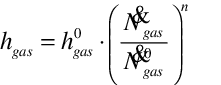
In several places the model is formulated to offer
different options. For example, the flow rate of process air
can be described either as a function of electrical power
produced or the fuel flow rate.
or
or
where,
 is an adjustment
factor,
is an adjustment
factor,
 ,
,
The Annex 42 fuel cell was implemented directly in
EnergyPlus. A sequential substitution method is used to handle
all the interactions between the different subsystems. The
main energy balance drawn for the fuel cell power module is
rearranged to put all the terms on the right hand side. The
enthalpy of the product gas stream is determined from this
energy balance. The Shomate equation is used to evaluate the
enthalpy and specific heat of the various streams. The
EnergyPlus implementation evaluates fluid properties using the
average temperature of inlet and outlet streams whereas the
Annex 42 specification often uses just the inlet temperature.
The Shomate equation is inverted using the regula falsi
numerical method available within EnergyPlus to calculate the
temperature of the product gases from their enthalpy.
Beausoleil-Morrison, I., A. Schatz, and F. Marechal. 2006.
A model for simulating the thermal and electrical production
of small-scale solid-oxide fuel cell cogeneration systems
within building simulation programs. HVAC & R
Research. Amer. Soc. Heating, Ref. Air-Conditioning Eng.
Inc. Atlanta, GA.
Beausoleil-Morrison, I., A. Weber, F. Marechal, and B.
Griffith. 2007. Specifications for Modelling Fuel Cell
Cogeneration Devices within Whole-Building Simulation
Programs. In Specifications for Modelling Fuel Cell and
Combustion-Based Residential Cogeneration Device within
Whole-Building Simulation Programs. I.
Beausoleil-Morrison and N. Kelly editors.
Draft report of Annex 42 of the International
Energy Agency ECBCS.
Custom Fuel Supply
for Generators[LINK]
The Generator:FuelSupply
input object in EnergyPlus implements a fairly comprehensive
capability to calculate properties of fuel mixtures from a
description of the molar composition of all the constituents.
The fuel supply modeling is based on the specifications
prepared by IEA Annex 42 for their generator models. This
modeling capability allows taking into consideration the exact
gas composition of local natural gas service. Or the user can
explore the implications of an various alternative fuels such
as alcohols or biogas. An unlimited number of possible
mixtures can be analyzed.
Gas phase thermochemistry calculations and data are
programmed into EnergyPlus to handle the set of constituents
listed in the table below. The relevant properties of each
fuel constituent, i, are calculated as a function of
temperature using the Shomate equation:
where,
 is the enthalpy
(J/kmol)
is the enthalpy
(J/kmol)
 is the molar enthalpy at
the standard state (J/kmol)
is the molar enthalpy at
the standard state (J/kmol)
 is the temperature of the
gas (K)
is the temperature of the
gas (K)
A, B, C, D, E, F, H are the coefficients for the Shomate
equation.
The lower heating value (LHV) of a fuel mixture is
calculated from the molar fractions using:
Where,
x is the number of carbon atoms
y is the number of hydrogen atoms
Similarly, the higher heating value (HHV) of the fuel
mixture is calculated using:
Where,
The Shomate coefficients used in EnergyPlus are listed in
the table below. Data source “NIST” indicates the data were
directly from Chemistry WebBook. Data source “CHEMKIN”
indicates the data were developed by curve fitting library
data for the CHEMKIN commercial program (which uses the
Gorden-McBride polynomial rather than the Shomate
formulation).
| Constituent |
A |
B |
C |
D |
E |
F |
H |
Source |
| N2 |
26.092 |
8.218801 |
-1.976141 |
0.159274 |
0.044434 |
-7.98923 |
0.0 |
NIST |
| O2 |
29.659 |
6.137261 |
-1.186521 |
0.09578 |
-0.219663 |
-9.861391 |
0.0 |
NIST |
| Ar |
20.786 |
2.8259E-7 |
-1.4642E-7 |
1.0921E-8 |
-3.6614E-8 |
-6.19735 |
0.0 |
NIST |
| CO2 |
24.99735 |
55.18696 |
-33.69137 |
7.948387 |
-0.136638 |
-403.6075 |
-393.5224 |
NIST |
| H2O(gas) |
29.0373 |
10.2573 |
2.81048 |
-0.95914 |
0.11725 |
-250.569 |
-241.8264 |
CHEMKIN |
| H2O(liq) |
-203.606 |
1523.29 |
-3196.413 |
2474.455 |
3.85533 |
-256.5478 |
-285.8304 |
NIST |
| H2 |
33.066178 |
-11.363417 |
11.432816 |
-2.772874 |
-0.158558 |
-9.9808 |
0.0 |
NIST |
| CH4 |
-0.703029 |
108.4773 |
-42.52157 |
5.862788 |
0.678565 |
-76.84376 |
-74.8731 |
NIST |
| C2H6 |
-3.03849 |
199.202 |
-84.9812 |
11.0348 |
0.30348 |
-90.0633 |
-83.8605 |
CHEMKIN |
| C3H8 |
-23.1747 |
363.742 |
-222.981 |
56.253 |
0.61164 |
-109.206 |
-103.855 |
CHEMKIN |
| C4H10 |
-5.24343 |
426.442 |
-257.955 |
66.535 |
-0.26994 |
-149.365 |
-133.218 |
CHEMKIN |
| C5H12 |
-34.9431 |
576.777 |
-338.353 |
76.8232 |
1.00948 |
-155.348 |
-146.348 |
CHEMKIN |
| C6H14 |
-46.7786 |
711.187 |
-438.39 |
103.784 |
1.23887 |
-176.813 |
-166.966 |
CHEMKIN |
| CH3OH |
14.1952 |
97.7218 |
-9.73279 |
-12.8461 |
0.15819 |
-209.037 |
-201.102 |
CHEMKIN |
| C2H5OH |
-8.87256 |
282.389 |
-178.85 |
46.3528 |
0.48364 |
-241.239 |
-234.441 |
CHEMKIN |
Beausoleil-Morrison, I., A. Weber, F.
Marechal, and B. Griffith. 2007. Specifications for Modelling
Fuel Cell Cogeneration Devices within Whole-Building
Simulation Programs. In Specifications for Modelling Fuel
Cell and Combustion-Based Residential Cogeneration Device
within Whole-Building Simulation Programs. I.
Beausoleil-Morrison and N. Kelly editors. Report of Annex 42
of the International Energy Agency ECBCS.
NIST. 2003. Chemistry WebBook, National Institute of
Standards and Technology Standard Reference Database Number
69, March 2003 Release,
http://webbook.nist.gov/chemistry/.
Gordon S. and B.J. McBride. 1971. Computer program for
calculation of complex chemical equilibrium composition,
rocket performance, incident and reflected shocks and
Chapman-Jouguet detonations. NASA SP-273.
The wind turbine (object Generator:WindTurbine) model is
intended to estimate the production of electric power of both
horizontal and vertical axis wind turbine systems. Due to the
cubic relationship between the wind speed and the power
produced by a wind turbine, the performance of these systems
is highly dependent on local wind conditions. However,
differences between typical meteorological year (TMY) wind
data attached to the simulation and local wind data at the
site where wind turbine system is installed typically appear.
The model thus estimates the air density and wind speed at the
particular height of the system and factors differences
between the wind speed from the TMY weather data and the local
wind speed. The weather data file should thus be included in
the simulation. The model also requires inputs of both an
annual average wind speed that represents accurate wind
profile at the location and the height where this annual
average wind speed was determined.
The model calculates the power production by both
horizontal axis wind turbines (HAWT) and vertical axis wind
turbines (VAWT) from generic mathematical equations.
Currently, a variable speed control scheme is available in
EnergyPlus. The model assumes constant power generation at the
rated power and the rated wind speed when the ambient wind
speed is between the rated wind speed and cut out wind speed.
The model does not attempt to model various types of
subsystems of the entire wind turbine system such as shafts,
generators and inverters due to computational convergence,
time, and usability. Instead, the total system efficiency
includes both conversion losses occurring during the DC-AC-DC
conversion processes and delivery losses.
Model Description[LINK]
The wind turbine is modeled as a generation component that
produces electricity and delivers it directly to buildings.
Wind turbine components are executed at the beginning of each
time step called by the HVAC manager, and the electric load
will be corrected with electricity from the wind turbine. The
model calculates electricity production that both HAWTs and
VAWTs produce from general mathematical equations. The model
then passes the electricity to the electric load center in
EnergyPlus at each HVAC system time step. The electric load
center then determines the whole building electrical demand,
deducting the power output by wind turbine along with any
power production by photovoltaic components from the total
electrical demand requested in the building. Excessive
production of electricity greater than needed from wind
turbine along with photovoltaic components is either sold or
stored as the user specifies.
The user must input the required information according to
the IO Reference Manual (ref: Generator:WindTurbine). The wind
turbine model in EnergyPlus requires a unique identifying name
and an availability schedule. The schedule name must refer to
a valid schedule type (range 0-1) and contain values of
fractional operation. Various inputs describes wind turbine
configuration such as rotor type, control type, rotor
diameter, overall height, and number of blades. Rated data
provided in the manufacturer’s literature determines overall
electricity production by using generic equations. These
inputs include rated power, rated wind speed, cut in wind
speed, cut out wind speed, fraction system efficiency, and
maximum tip speed ratio. Two inputs such as annual local
average wind speed and height for local average wind speed
define local wind conditions at a specific location so that
the model predicts wind speed and air density at the height of
the wind turbine at the location.
HAWT systems need a maximum power coefficient and empirical
power coefficient parameters C1 through
C6. The maximum power coefficient controls
overall performance of the rotor which defines the power
extraction efficiency from the ambient air stream. The model
predicts power generation more accurately when the user inputs
the empirical power coefficients C1
through C6 for a specific wind turbine.
Three additional inputs for VAWT system are required. The
model requests blade lift and drag coefficients corresponding
to the maximum tip speed ratio so that tangential and normal
force coefficients are obtained. Blade chord area is also
requested for calculating forces on a single blade.
Simulation and Control[LINK]
Given the inputs needed, the wind turbine model analyzes
local wind speed since wind speed is critical to determine the
production of electricity of wind turbine systems. To minimize
uncertainty involved with wind data, it factors differences
between annual average wind speed from weather data and local
annual average wind speed at the particular height of the
local meteorological station. It reads annual average wind
speed from statistical weather file that is automatically
copied during the simulation. Note that the user should attach
a weather data to the simulation (for a design day simulation,
the wind speed data from the design day description is used).
This annual average wind speed is converted into a wind speed
at the height at which local annual average wind speed that
the user inputs is measured and then factored as:
Note that the wind speed factor Fv of
1.0 is assigned, if the user does not input the local wind
conditions or the weather data file is not attached to the
simulation.
The local air density can be obtained by using EnergyPlus
psychrometric functions as follows:
The model converts TMY wind speed into a wind speed at the
specific height of the wind turbine rotor
(Vz) at the location by using EnergyPlus
function as:
The local wind speed at the rotor height
(VLocal) at the location is thus:
The tip speed ratio (TSR) can be obtained as:
Horizontal Axis Wind
Turbine[LINK]
Once the local wind speed and air density are determined,
the model calculates electrical power produced by a wind
turbine system according to the rotor type. For HAWT systems,
two different approximations are available. The model uses an
analytical approximation when the user inputs all six
empirical coefficient parameters C1
through C6. The equations that define the
analytical approximation are:
Note that the model allows changing the rotor speed to meet
the maximum tip speed ratio at each time step. That is, the
tip speed ratio calculated is limited by the maximum tip speed
ratio. Similarly, the power coefficient calculated is also set
to the maximum if the calculated is greater than the
maximum.
Assuming maximum of rotor angle, i.e. zero, the power
production of the wind turbine is thus obtained by:
The model assumes the simple approximation, if any of
empirical power coefficient parameters is not input. The power
production of wind turbine is directly obtained from the
kinetic energy equation:
Here, the model defines PW as rated
power output at the rated wind speed, if either the power
production of wind turbine or local wind speed is greater than
the rated power or rated wind speed, respectively. The power
coefficient in this particular case is thus recalculated
as:
The overall power production that includes conversion loss
and delivery loss is thus:
Vertical Axis Wind
Turbine[LINK]
If tip speed ratio at the time step is greater than the
maximum tip speed ratio, the model estimates actual rotor
speed at the time step as:
The model then employs general mathematical expressions for
the aerodynamic analysis of straight-bladed Darrieus-type
VAWTs to predict the power production by VAWTs. Assuming
quasi-steady state, the induced wind speed
(Va) on the rotor is defined as:
The chordal velocity (Vc), normal
velocity (Vn), and relative flow velocity
(W) as shown in figure above can be expressed as:
The expression for the non-dimensional angle of attack
(α) with no consideration of blade pitch is:
The tangential and normal force coefficients, respectively,
are expressed as:
The net tangential and normal forces are obtained from the
following expressions:
Average tangential force on a single blade can be defined
as:
Substituting the values of Ft and
arranging tangential force on azimuth angle,  , equation above can be written
as:
, equation above can be written
as:
The expression of the total torque for the number of blades
is defined as:
The power production of wind turbine is thus:
The model also defines PW as the rated
power output at the rated wind speed, if either the power
production of wind turbine or local wind speed is greater than
the rated power.
The overall power production delivered from a wind turbine
system is thus:
Nomenclature for Wind Turbine model
Variable
Description
Units
AR
swept area of rotor
m2
AC
blade chord area
m2
a
site wind exponent, 0.22
amet
wind exponent, 0.14
Cd
blade drag coefficient, 0.9
Cl
blade lift coefficients, 0.05
Cn
normal force coefficient
Cp
power coefficient (performance coefficient)
Ct
tangential force coefficient
C1-6
empirical power coefficient parameters
go
standard gravity
m/s2
Fn
normal force in radial direction
N.m (J)
Ft
tangential force
N.m (J)
Fta
average tangential force
N.m (J)
Fv
wind speed factor
H
height of local wind speed measurement
m
Hmet
height of turbine, 10
m
N
number of blade
P
overall power production delivered to building
W
PLocal
outdoor static air pressure at rotor height
Pa
PW
wind turbine power produced
W
Q
overall torque
N.m
R
turbine radius
m
TLocal
local air temperature at rotor height
℃
v
ambient wind speed
m/s
v1
upstream wind speed
m/s
v2
wind speed on the turbine
m/s
v3
downstream wake velocity
m/s
Va
induced velocity
m/s
VAnnualAvg
annual average wind speed from TMY weather data
m/s
VLocal
local wind speed at the location of the system
m/s
VLocalTMY
annual average wind speed converted at the local station
height
m/s
Vc
chordal velocity component
m/s
Vn
normal velocity component
m/s
VZ
wind speed adjusted at rotor height
m/s
W
relative flow velocity
m/s
Z
height of wind turbine rotor
m
α
blade angle of attack
deg
θ
azimuth angle in VAWT and pitch angle in HAWT
deg
ρLocal
local density of air at rotor height
kg/m3
ω
angular velocity of turbine
rad/s
ωLocal
local humidity ratio at rotor height
kg-H2O/kg-air
x
exponent, 1.5
λ
tip speed ratio
λi
tip speed ratio at the ith pitch
δmet
wind boundary layer thickness of meteorological station,
270
m
δ
site boundary layer thickness, 370
m
η
wind turbine system efficiency
Siegfried Heier. 2006. Grid Integration of Wind Energy
Conversion Systems, Second Edition. Wiley, Chap. 2,
pp.31-44.
Mazharul Islam, David S.K. Ting and Amir Fartaj. 2008.
Aerodynamic Models for Darrieus-type Sraight-bladed Vertical
Axis Wind Turbines. Renewable & Sustainable Energy
Reviews, Volume 12, pp.1087-1109.
ASHRAE. 2005. Handbook of Fundamentals, pp 16.3-16.4,
Atlanta: ASHRAE.

Generators[LINK]
Internal Cumbustion Engine[LINK]
The engine-driven generator model was originally developed for the BLAST program and was subsequently adapted for use in EnergyPlus. The model uses the following set of equations all of which are quadratic fits to the PLR (Part Load Ratio) of the generator. The coefficients must be derived from manufacturers data.
The electrical load and engine generator nominal load capacity are used to compute the part load ratio.
The exhaust gas temp and flow rate are used if a stack heat exchanger is used to recover waste heat from the exhaust. This temperature is the inlet temperature to the heat exchanger which is modeled in a UA-effectiveness form:
The exhaust flow rate is then calculated as:
where Treference is the reference temperature for the fuel lower heating value, and is given as 25°C in manufacturer’s data, and
Finally heat recovered from the lube oil and the water jacket are accounted for as follows:
The manufacturer must supply the recoverable water jacket heat, lube oil heat and exhaust heat and associated fuel consumption for a range of load conditions. This data is then fit to the PLR to obtain the fifteen a,b,c,d, and e coefficients.
Turbine Generator[LINK]
The combustion turbine generator model was originally developed for the BLAST program and was subsequently adapted for use in EnergyPlus. The model uses the following set of equations all of which are equation fits to the PLR (Part Load Ratio) of the generator and the entering air temperature. The coefficients must be derived from manufacturers data. For electric power generated in Watts, the fuel input rate is calculated in J/s.
The electrical load and engine generator nominal load capacity are used to compute the part load ratio.
The temperature difference shows the deviation of ambient air temperature from the manufacturers design air temperature.
A second curve fit calculates the exhaust temperature (C) by multiplying the exhaust temperature (C) for a particular part load by a correction factor based on the deviation from design temperature.
The exhaust gas temp is used if a stack heat exchanger is used to recover waste heat from the exhaust. This temperature is the inlet temperature to the heat exchanger which is modeled in a UA-effectiveness form:
Where the design minimum exhaust temperature is a user input to the model and the exhaust mass flow rate and the UA are fit from manufacturers data as follows:
Finally, heat recovered from the lube oil is accounted for as follows:
Microturbine Generator[LINK]
Microturbine generators are small combustion turbines that produce electricity on a relatively small scale (e.g., 25kW to 500kW). This model uses nominal performance at reference conditions along with several modifier curves to determine electrical power output and fuel use at non-reference conditions. The modifier curve coefficients must be derived from manufacturers data. Standby and ancillary power can also be taken into account.
Exhaust air energy recovery for heating water can be also be modeled. Similar to electrical power output, thermal power (heat recovery to water) output is calculated using nominal performance at reference conditions with modifier curves to account for variations at non-reference conditions. The ElectricLoadCenter:Generators and ElectricLoadCenter:Distribution objects are used to define the availability and control of the electric generators included in the simulation (ref. ElectricLoadCenter:Generators and ElectricLoadCenter:Distribution).
For each simulation time step that the generator is being asked to operate (i.e., produce electrical power as determined by the ElectricLoadCenter), the full load electrical output of the generator is determined using the user-defined reference electrical power output along with a bi-quadratic modifier curve to account for differences in the combustion air inlet temperature and elevation for the current simulation time step compared to the reference temperature and elevation (i.e., the modifier curve should evaluate to 1.0 at the reference combustion air inlet temperature and reference elevation).
where:
The full load electrical power output of the generator is then checked against the minimum and maximum full load electrical power outputs specified by the user:
The actual (operating) electrical power output from the generator is determined next based on the load requested by the Electric Load Center, the generator’s minimum and maximum part-load ratios, and the ancillary power.
where:
The generator’s electrical efficiency is then calculated based on the user-specified reference electrical efficiency (lower heating value [LHV] basis) and two electrical efficiency modifier curves.
where:
The fuel energy consumption rate (LHV Basis) is then calculated as follows:
where:
If ElecEffOperating is equal to zero, then POperating and ~~are set to zero. The fuel mass
flow rate is then calculated.
~~are set to zero. The fuel mass
flow rate is then calculated.
where:
LHV = Fuel Lower Heating Value, user input (kJ/kg)
The ancillary power is calculated next using the user-specified ancillary power and ancillary power modifier curve. The ancillary power modifier curve is a quadratic function with the generator’s fuel mass flow rate as the independent variable. If an ancillary power modifier curve is not specified in the input file, the modifier is assumed to be 1.0 and the ancillary power will be constant throughout the simulation.
where:
If ancillary power is constant for the simulation (e.g., no modifier curve defined), then the calculations continue as described below. However, if an ancillary power modifier curve has been defined, then the calculations described above for PElecOperating, ElecEffOperating, ~~and
PAncillary,Operating are recalculated in
sequence until the solution converges.
~~and
PAncillary,Operating are recalculated in
sequence until the solution converges.
The generator’s “net” electrical power output is calculated as the difference between the generator’s actual power output and the ancillary electric power as follows.
where:
The fuel energy consumption rate (higher heating value basis) for the generator is then calculated as follows:
where:
Standby electrical power may also be modeled to simulate controls or other parasitics used by the generator. The standby power is calculated only when the generator is not operating (i.e., Load from the Electric Load Center is zero). If the generator operates for a given timestep (i.e., Load > 0.0), the standby power is set equal to 0.
where:
Report variables for electric energy produced, electric efficiency (LHV basis), fuel consumption (HHV basis), standby electric consumption and ancillary electric consumption are calculated as follows:
where:
TimeStepSys = HVAC system simulation time step (hr)
In addition to calculating electric power production and fuel usage, the model is able to determine thermal power (heat recovery) output for heating water. For this case, the water flow rate through the heat recovery heat exchanger is established first. If the Heat Recovery Water Flow Operating Mode (user input) is set to Plant Control, then the Reference Heat Recovery Water Flow Rate (user input) is requested whenever the generator operates (constant value), but the actual flow rate may be restricted by other plant components (e.g., pump). If the Heat Recovery Water Flow Operating Mode is set to Internal Control, then the requested water flow when the generator operates is determined by the Reference Heat Recovery Water Flow Rate and a flow rate modifier curve.
where:
The methodology for determining thermal power (heat recovery to water) is similar to that used for calculating electric power production. The generator’s steady-state thermal efficiency is calculated based on the user-specified reference thermal efficiency (LHV basis) and a thermal efficiency modifier curve.
where:
The steady-state thermal power produced (heat recovery rate) is then calculated:
The actual (operating) thermal power is then calculated using the steady-state thermal power and three modifier curves:
where:
The heat recovery output water temperature is then calculated.
where:
If the calculated heat recovery outlet water temperature exceeds to Maximum Heat Recovery Water Temperature (user input), then the outlet water temperature is reset to the maximum temperature (user input) and the thermal power is recalculated.
If combustion air inlet and outlet node names are specified in the input, along with exhaust air flow rate and exhaust air temperature information, then the model calculates the exhaust air conditions for each simulation time step. The exhaust air mass flow rate is first calculated based on the Reference Exhaust Air Mass Flow Rate, two modifier curves and an air density adjustment. Since fans are volumetric flow devices, the ratio of the air density at actual inlet air conditions to air density at reference inlet air conditions is used as an adjustment factor.
where:
In an analogous fashion, the exhaust air temperature is calculated using the Nominal (reference) Exhaust Air Outlet Temperature and two modifier curves.
where:
The above calculations for exhaust air outlet temperature assume no heat recovery to water is being done. If thermal power (water heating) is being produced, then the exhaust air outlet temperature is recalculated as follows:
where:
The exhaust air outlet humidity ratio is also calculated.
where:
The remaining report variables are calculated as follows.
where:
Micro-Cogenerator[LINK]
The input object Generator:MicroCHP provides a model that is a direct implementation of a model developed by IEA Annex 42 – The Simulation of Building-Integrated Fuel Cell and Other Cogeneration Systems (FC+COGEN-SIM). Annex 42 was formed as a working group within the International Energy Agency (IEA) program on Energy Conservation in Buildings and Community Systems (ECBCS). A full description of the model specification can be found in the report by Subtask B of FC+COGEN-SIM with the title “Specifications for Modelling Fuel Cell and Combustion-Based Residential Cogeneration Device within Whole-Building Simulation Programs.” The “Micro CHP” model in EnergyPlus is the one referred to as “A Generic Model for Combustion-based Residential Cogeneration Devices.”
The Micro CHP model is a straightforward empirical model with the exception that it is dynamic with respect to thermal heat recovery where performance is cast as a function of engine temperature. It is also dynamic with respect to possible warm up and cool down periods that may affect the ability of the generator to deliver the requested power. The relevant model equations are:
where,
The functional forms for and
and  are 2nd order
trivariate polynomials with all of the cross terms.
are 2nd order
trivariate polynomials with all of the cross terms.
EnergyPlus solves these for state values for the engine mass temperature, , and the
outlet plant node,
, and the
outlet plant node,  , in the
following manner. The last two equations are interrelated but
otherwise ordinary differential equations with the general
form
, in the
following manner. The last two equations are interrelated but
otherwise ordinary differential equations with the general
form
and have analytical solution
The engine temperature at the current timestep is calculated using
The plant node outlet fluid temperature (heat recovered) is solved using
The interrelation of these two is handled by sequential substitution using an iteration scheme that alternates between calculations of and
and  . The iteration loop exits once
the energy is determined to be balanced using the following
criteria:
. The iteration loop exits once
the energy is determined to be balanced using the following
criteria:
Number of iterations > 3\
The Micro CHP model has a number of different operating modes. The operating mode for a given system timestep is determined from the mode during the previous timestep, user inputs, and high-level controls from elsewhere in EnergyPlus. The operating mode is reported for the state at the end of each timestep. The following table summarizes the various operating modes and the criteria for switching to a new mode for any given timestep. The EnergyPlus implementation adds the “Off” mode to the modes specified by Annex 42 which corresponds to the unit being scheduled to be unavailable. The difference between OFF and Standby modes determines whether or not standby power is consumed.
For timesteps where the generator switches from warm up mode to normal mode in the middle of the timestep, part load ration values are calculated for the portion of the time step that the generator is in normal operation.
The engine and heat recovery thermal conditions are modeled for all modes so, for example, an engine that is off but still warm could provide some hot water recovery.
The engine model can use an arbitray fuel mixture that is defined by the user – see the entry for Generator:FuelSupply.
References[LINK]
Kelly, N. and A. Ferguson. 2007. A Generic Model Specification for Combustion-based Residential Cogeneration Devices. In Specifications for Modelling Fuel Cell and Combustion-Based Residential Cogeneration Device within Whole-Building Simulation Programs. I. Beausoleil-Morrison and N. Kelly editors. Draft report of Annex 42 of the International Energy Agency ECBCS.
Fuel Cell Cogenerator[LINK]
The Generator:FuelCell input objects provides a model which is a direct implementation of a model developed by IEA Annex 42 – The Simulation of Building-Integrated Fuel Cell and Other Cogeneration Systems (FC+COGEN-SIM). Annex 42 was formed as a working group within the International Energy Agency (IEA) program on Energy Conservation in Buildings and Community Systems (ECBCS). A full description of the model specification can be found in the report by Subtask B of FC+COGEN-SIM with the title “Specifications for Modelling Fuel Cell and Combustion-Based Residential Cogeneration Device within Whole-Building Simulation Programs.” The “Specifications for Modelling Fuel Cell Cogeneration Devices within Whole-Building Simulation Programs.”
The Annex 42 Fuel Cell model is characterized as a “grey box” empirical model where a mixture of thermodynamic principles and empirical performance maps are used to model the cogeneration performance of a fairly complex device with many individual subsystems. In EnergyPlus, the individual subsystems are separate into individual input objects such as Generator:FuelCell:PowerModule or Generator:FuelCell:ExhaustGasToWaterHeatExchanger. The resulting model is relatively complex requiring on the order of one hundred inputs. The model is not for the faint of heart; this model is far more involved than most component models in building simulation. This stems from the fact that fuel cell cogenerators are complicated devices that interact with the built environment in a number of ways. Fuel cells could drawn in gas/fuel, air, and water with as many as six separate streams. In addition to electricity and heated water, they also give off heat in the form of convection and radiation and exhaust air out of the zone. The devices may take a long time to start up and include storage to follow loads rather than attempt to vary the power the fuel cell. The fuel cell model allows examining system level interactions over annual timeframes that include all the important interactions with a building’s energy and comfort systems.
The Annex 42 fuel cell model is described more thoroughly in the references (see below). Here we provide a summary of the relevant model equations which are taken from the Annex 42 model specification. The first equation is the main energy balance for the fuel cell power module (includes the fuel reformation and fuel cell stacks). This energy balance is used to model the enthalpy of the product gases that leave the fuel cell power module.
The remaining equations describe various terms and the balance of systems. The electrical efficiency is modeled using:
In several places the model is formulated to offer different options. For example, the flow rate of process air can be described either as a function of electrical power produced or the fuel flow rate.
or
or
where,
The Annex 42 fuel cell was implemented directly in EnergyPlus. A sequential substitution method is used to handle all the interactions between the different subsystems. The main energy balance drawn for the fuel cell power module is rearranged to put all the terms on the right hand side. The enthalpy of the product gas stream is determined from this energy balance. The Shomate equation is used to evaluate the enthalpy and specific heat of the various streams. The EnergyPlus implementation evaluates fluid properties using the average temperature of inlet and outlet streams whereas the Annex 42 specification often uses just the inlet temperature. The Shomate equation is inverted using the regula falsi numerical method available within EnergyPlus to calculate the temperature of the product gases from their enthalpy.
References[LINK]
Beausoleil-Morrison, I., A. Schatz, and F. Marechal. 2006. A model for simulating the thermal and electrical production of small-scale solid-oxide fuel cell cogeneration systems within building simulation programs. HVAC & R Research. Amer. Soc. Heating, Ref. Air-Conditioning Eng. Inc. Atlanta, GA.
Beausoleil-Morrison, I., A. Weber, F. Marechal, and B. Griffith. 2007. Specifications for Modelling Fuel Cell Cogeneration Devices within Whole-Building Simulation Programs. In Specifications for Modelling Fuel Cell and Combustion-Based Residential Cogeneration Device within Whole-Building Simulation Programs. I. Beausoleil-Morrison and N. Kelly editors. Draft report of Annex 42 of the International Energy Agency ECBCS.
Custom Fuel Supply for Generators[LINK]
The Generator:FuelSupply input object in EnergyPlus implements a fairly comprehensive capability to calculate properties of fuel mixtures from a description of the molar composition of all the constituents. The fuel supply modeling is based on the specifications prepared by IEA Annex 42 for their generator models. This modeling capability allows taking into consideration the exact gas composition of local natural gas service. Or the user can explore the implications of an various alternative fuels such as alcohols or biogas. An unlimited number of possible mixtures can be analyzed.
Gas phase thermochemistry calculations and data are programmed into EnergyPlus to handle the set of constituents listed in the table below. The relevant properties of each fuel constituent, i, are calculated as a function of temperature using the Shomate equation:
where,
A, B, C, D, E, F, H are the coefficients for the Shomate equation.
The lower heating value (LHV) of a fuel mixture is calculated from the molar fractions using:
Where,
x is the number of carbon atoms
y is the number of hydrogen atoms
Similarly, the higher heating value (HHV) of the fuel mixture is calculated using:
Where,
The Shomate coefficients used in EnergyPlus are listed in the table below. Data source “NIST” indicates the data were directly from Chemistry WebBook. Data source “CHEMKIN” indicates the data were developed by curve fitting library data for the CHEMKIN commercial program (which uses the Gorden-McBride polynomial rather than the Shomate formulation).
References[LINK]
Beausoleil-Morrison, I., A. Weber, F. Marechal, and B. Griffith. 2007. Specifications for Modelling Fuel Cell Cogeneration Devices within Whole-Building Simulation Programs. In Specifications for Modelling Fuel Cell and Combustion-Based Residential Cogeneration Device within Whole-Building Simulation Programs. I. Beausoleil-Morrison and N. Kelly editors. Report of Annex 42 of the International Energy Agency ECBCS.
NIST. 2003. Chemistry WebBook, National Institute of Standards and Technology Standard Reference Database Number 69, March 2003 Release, http://webbook.nist.gov/chemistry/.
Gordon S. and B.J. McBride. 1971. Computer program for calculation of complex chemical equilibrium composition, rocket performance, incident and reflected shocks and Chapman-Jouguet detonations. NASA SP-273.
Wind Turbine[LINK]
Overview[LINK]
The wind turbine (object Generator:WindTurbine) model is intended to estimate the production of electric power of both horizontal and vertical axis wind turbine systems. Due to the cubic relationship between the wind speed and the power produced by a wind turbine, the performance of these systems is highly dependent on local wind conditions. However, differences between typical meteorological year (TMY) wind data attached to the simulation and local wind data at the site where wind turbine system is installed typically appear. The model thus estimates the air density and wind speed at the particular height of the system and factors differences between the wind speed from the TMY weather data and the local wind speed. The weather data file should thus be included in the simulation. The model also requires inputs of both an annual average wind speed that represents accurate wind profile at the location and the height where this annual average wind speed was determined.
The model calculates the power production by both horizontal axis wind turbines (HAWT) and vertical axis wind turbines (VAWT) from generic mathematical equations. Currently, a variable speed control scheme is available in EnergyPlus. The model assumes constant power generation at the rated power and the rated wind speed when the ambient wind speed is between the rated wind speed and cut out wind speed. The model does not attempt to model various types of subsystems of the entire wind turbine system such as shafts, generators and inverters due to computational convergence, time, and usability. Instead, the total system efficiency includes both conversion losses occurring during the DC-AC-DC conversion processes and delivery losses.
Model Description[LINK]
The wind turbine is modeled as a generation component that produces electricity and delivers it directly to buildings. Wind turbine components are executed at the beginning of each time step called by the HVAC manager, and the electric load will be corrected with electricity from the wind turbine. The model calculates electricity production that both HAWTs and VAWTs produce from general mathematical equations. The model then passes the electricity to the electric load center in EnergyPlus at each HVAC system time step. The electric load center then determines the whole building electrical demand, deducting the power output by wind turbine along with any power production by photovoltaic components from the total electrical demand requested in the building. Excessive production of electricity greater than needed from wind turbine along with photovoltaic components is either sold or stored as the user specifies.
Input and Data[LINK]
The user must input the required information according to the IO Reference Manual (ref: Generator:WindTurbine). The wind turbine model in EnergyPlus requires a unique identifying name and an availability schedule. The schedule name must refer to a valid schedule type (range 0-1) and contain values of fractional operation. Various inputs describes wind turbine configuration such as rotor type, control type, rotor diameter, overall height, and number of blades. Rated data provided in the manufacturer’s literature determines overall electricity production by using generic equations. These inputs include rated power, rated wind speed, cut in wind speed, cut out wind speed, fraction system efficiency, and maximum tip speed ratio. Two inputs such as annual local average wind speed and height for local average wind speed define local wind conditions at a specific location so that the model predicts wind speed and air density at the height of the wind turbine at the location.
HAWT systems need a maximum power coefficient and empirical power coefficient parameters C1 through C6. The maximum power coefficient controls overall performance of the rotor which defines the power extraction efficiency from the ambient air stream. The model predicts power generation more accurately when the user inputs the empirical power coefficients C1 through C6 for a specific wind turbine. Three additional inputs for VAWT system are required. The model requests blade lift and drag coefficients corresponding to the maximum tip speed ratio so that tangential and normal force coefficients are obtained. Blade chord area is also requested for calculating forces on a single blade.
Simulation and Control[LINK]
Given the inputs needed, the wind turbine model analyzes local wind speed since wind speed is critical to determine the production of electricity of wind turbine systems. To minimize uncertainty involved with wind data, it factors differences between annual average wind speed from weather data and local annual average wind speed at the particular height of the local meteorological station. It reads annual average wind speed from statistical weather file that is automatically copied during the simulation. Note that the user should attach a weather data to the simulation (for a design day simulation, the wind speed data from the design day description is used). This annual average wind speed is converted into a wind speed at the height at which local annual average wind speed that the user inputs is measured and then factored as:
Note that the wind speed factor Fv of 1.0 is assigned, if the user does not input the local wind conditions or the weather data file is not attached to the simulation.
The local air density can be obtained by using EnergyPlus psychrometric functions as follows:
The model converts TMY wind speed into a wind speed at the specific height of the wind turbine rotor (Vz) at the location by using EnergyPlus function as:
The local wind speed at the rotor height (VLocal) at the location is thus:
The tip speed ratio (TSR) can be obtained as:
Horizontal Axis Wind Turbine[LINK]
Once the local wind speed and air density are determined, the model calculates electrical power produced by a wind turbine system according to the rotor type. For HAWT systems, two different approximations are available. The model uses an analytical approximation when the user inputs all six empirical coefficient parameters C1 through C6. The equations that define the analytical approximation are:
Note that the model allows changing the rotor speed to meet the maximum tip speed ratio at each time step. That is, the tip speed ratio calculated is limited by the maximum tip speed ratio. Similarly, the power coefficient calculated is also set to the maximum if the calculated is greater than the maximum.
Assuming maximum of rotor angle, i.e. zero, the power production of the wind turbine is thus obtained by:
The model assumes the simple approximation, if any of empirical power coefficient parameters is not input. The power production of wind turbine is directly obtained from the kinetic energy equation:
Here, the model defines PW as rated power output at the rated wind speed, if either the power production of wind turbine or local wind speed is greater than the rated power or rated wind speed, respectively. The power coefficient in this particular case is thus recalculated as:
The overall power production that includes conversion loss and delivery loss is thus:
Vertical Axis Wind Turbine[LINK]
If tip speed ratio at the time step is greater than the maximum tip speed ratio, the model estimates actual rotor speed at the time step as:
The model then employs general mathematical expressions for the aerodynamic analysis of straight-bladed Darrieus-type VAWTs to predict the power production by VAWTs. Assuming quasi-steady state, the induced wind speed (Va) on the rotor is defined as:
The chordal velocity (Vc), normal velocity (Vn), and relative flow velocity (W) as shown in figure above can be expressed as:
The expression for the non-dimensional angle of attack (α) with no consideration of blade pitch is:
The tangential and normal force coefficients, respectively, are expressed as:
The net tangential and normal forces are obtained from the following expressions:
Average tangential force on a single blade can be defined as:
Substituting the values of Ft and arranging tangential force on azimuth angle, , equation above can be written
as:
, equation above can be written
as:
The expression of the total torque for the number of blades is defined as:
The power production of wind turbine is thus:
The model also defines PW as the rated power output at the rated wind speed, if either the power production of wind turbine or local wind speed is greater than the rated power.
The overall power production delivered from a wind turbine system is thus:
Nomenclature for Wind Turbine model
Variable
Description
Units
AR
swept area of rotor
m2
AC
blade chord area
m2
a
site wind exponent, 0.22
amet
wind exponent, 0.14
Cd
blade drag coefficient, 0.9
Cl
blade lift coefficients, 0.05
Cn
normal force coefficient
Cp
power coefficient (performance coefficient)
Ct
tangential force coefficient
C1-6
empirical power coefficient parameters
go
standard gravity
m/s2
Fn
normal force in radial direction
N.m (J)
Ft
tangential force
N.m (J)
Fta
average tangential force
N.m (J)
Fv
wind speed factor
H
height of local wind speed measurement
m
Hmet
height of turbine, 10
m
N
number of blade
P
overall power production delivered to building
W
PLocal
outdoor static air pressure at rotor height
Pa
PW
wind turbine power produced
W
Q
overall torque
N.m
R
turbine radius
m
TLocal
local air temperature at rotor height
℃
v
ambient wind speed
m/s
v1
upstream wind speed
m/s
v2
wind speed on the turbine
m/s
v3
downstream wake velocity
m/s
Va
induced velocity
m/s
VAnnualAvg
annual average wind speed from TMY weather data
m/s
VLocal
local wind speed at the location of the system
m/s
VLocalTMY
annual average wind speed converted at the local station height
m/s
Vc
chordal velocity component
m/s
Vn
normal velocity component
m/s
VZ
wind speed adjusted at rotor height
m/s
W
relative flow velocity
m/s
Z
height of wind turbine rotor
m
α
blade angle of attack
deg
θ
azimuth angle in VAWT and pitch angle in HAWT
deg
ρLocal
local density of air at rotor height
kg/m3
ω
angular velocity of turbine
rad/s
ωLocal
local humidity ratio at rotor height
kg-H2O/kg-air
x
exponent, 1.5
λ
tip speed ratio
λi
tip speed ratio at the ith pitch
δmet
wind boundary layer thickness of meteorological station, 270
m
δ
site boundary layer thickness, 370
m
η
wind turbine system efficiency
References[LINK]
Siegfried Heier. 2006. Grid Integration of Wind Energy Conversion Systems, Second Edition. Wiley, Chap. 2, pp.31-44.
Mazharul Islam, David S.K. Ting and Amir Fartaj. 2008. Aerodynamic Models for Darrieus-type Sraight-bladed Vertical Axis Wind Turbines. Renewable & Sustainable Energy Reviews, Volume 12, pp.1087-1109.
ASHRAE. 2005. Handbook of Fundamentals, pp 16.3-16.4, Atlanta: ASHRAE.
Documentation content copyright © 1996-2026 The Board of Trustees of the University of Illinois and the Regents of the University of California through the Ernest Orlando Lawrence Berkeley National Laboratory. All rights reserved. EnergyPlus is a trademark of the US Department of Energy.
This documentation is made available under the EnergyPlus Open Source License v1.0.