Chilled-Water-Based
Air Cooling Coil[LINK]
The input object Coil:Cooling:Water
is simpler than the detailed geometry model. The simple model
provides a good prediction of the air and water outlet
conditions without requiring the detailed geometric input
required for the detailed model. A greatly simplified
schematic of enthalpy and temperature conditions in a counter
flow cooling/dehumidifying coil is shown in the schematic
Figure 150. The input required to model the coil includes only
a set of thermodynamic design inputs, which require no
specific manufacturer’s data. The coil simulation model is
essentially a modification of one presented by Elmahdy and
Mitalas (1977), TRNSYS, 1990 and Threlkeld, J.L. 1970. The
model calculates the UA values required for a Dry, Wet and
Part Wet & Part Dry Coil and iterates between the Dry and
Wet Coil to output the fraction wet. There are two modes of
flow operation for this model: Cross Flow, which is widely
applicable in HVAC systems and the second being Counter flow
mode. The default value in program is set up for Counter Flow.
In addition the coil has two modes of analysis: Simple
Analysis and Detailed Analysis. The Simple analysis mode
operates the coil as either wet or dry while the detailed mode
simulates the coil as part wet part-dry. While the detailed
mode provides more accurate results, it is significantly
slower than the simple model. The simple mode gives good
results for an annual simulation but will not be adequate for
a time step performance analysis.
Heat Transfer and
Energy Balance[LINK]
The cooling coil may be completely dry, completely wet with
condensation, or it may have wet and dry sections. The actual
condition of the coil surface depends on the humidity and
temperature of the air passing over the coil and the coil
surface temperature. The part-dry part-wet case represents the
most general scenario for the coil surface conditions. There
are subroutines present in the model for both the dry and wet
regions of the coil, and a subroutine that iterates between
the dry and wet subroutines to calculate the fraction of the
coil surface that is wet. For each region the heat transfer
rate from air to water may be defined by the rate of enthalpy
change in the air and in the water. The rates must balance
between each medium for energy to be conserved.
Model Description[LINK]
The Model has two blocks: 1st = Design Block
with the Design Inputs. This block calculates the Design
U-Factor Times Area Value (UA) values required by the model.
Using these UA values the model simulates the operating
conditions. The operating block is the one containing the
operating conditions, the conditions at which the coil
operates. Following is the list of Design and Operating inputs
and subsequently the Design and Operating variables used in
the model.
Design Inputs (User Inputs)
| Input Field |
Description |
| DesWaterVolFlowRate: |
Maximum Water Volume Flow
Rate |
| DesAirVolFlowRate: |
Maximum Air Volume Flow
Rate |
| DesInletWaterTemp: |
Inlet Water Temperature at
Design Condition |
| DesInletAirTemp: |
Inlet Air Temperature at Design
Condition |
| DesOutletAirTemp: |
Outlet Air Temperature at Design
Condition |
| DesInletAirHumRat: |
Inlet Air Humidity Ratio at
Design Conditions |
| DesOutletAirHumRat: |
Outlet Air Humidity Ratio at
Design Conditions. |
Operating Conditions (From Nodes – not user
inputs)
| Condition Variable |
Description |
| InletWaterMassFlowRate: |
Entering Water Mass Flow Rate at
operating condition |
| InletWaterTemp: |
Inlet Water Temperature at
operating condition |
| InletAirMassFlowRate: |
Entering Air Mass Flow Rate at
operating condition |
| InletAirTemp: |
Inlet Air Temperature at
operating condition |
| InletAirHumRat: |
Entering air humidity ratio at
operating conditions |
The various U-Factor Times Area values (UA) required by
this model are calculated from the above inputs, which are
explained later in the document. The various UA are:
UA Descriptions of Model
| UA Variable Name |
Description |
| CoilUATotal: |
Overall heat transfer
coefficient (W/C) |
| CoilUAInternal: |
Overall internal UA (W/C) |
| CoilUAExternal: |
Overall external UA (W/C) |
| CoilUInternal: |
Internal overall heat transfer
coefficient (W/m2∙C) |
| CoilUWetExternal: |
Wet part external overall heat
transfer coefficient (W/m2∙C) |
| CoilUDryExternal: |
Dry part external overall heat
transfer coefficient (W/m2∙C) |
The UA values are calculated assuming a wet coil at the
design conditions. Following are a few important calculations
to understand the working of the model. The model is basically
divided into two blocks: the Design Block and the Operating
Block.
The Design Block is a one time calculation. The aim of the
Design Block is to calculate the Coil UA for use in the
operating Block.
The design block has the code for calculating the six Coil
UA values required by the operating block. Reasonable
assumptions have been made in the calculations to maintain the
simplicity of the model.
Heat transfer ina wet coil model is based on enthalpy
rather than temperature to take into account latent effects.
While heat transfer rates are commonly expressed as the
product of an overall heat transfer coefficient, UA, and a
temperature difference, the use of enthalpy-based heat
transfer calculations requires an enthalpy-based heat transfer
coefficient which we denote as DesUACoilTotalEnth and hence
the equation.
Q = DesUACoilTotalEnth * (Hair,mean -
Hwater,mean). The value of Q is calculated using
product of air mass flow rate and difference in inlet and
outlet air enthalpies at design conditions.
The relation between the enthalpy-based UA and the
temperature-based UA is DesUACoilTotalEnth = CoilUA /
Cp. CoilUA is the conventional heat transfer
coefficient and Cp = specific heat of the air.
We need the following quantities for our design
calculations. The Psy functions are the EnergyPlus
built-in psychrometric functions.
We now calculate the design coil bypass factor. The bypass
factor is not used in subsequent calculations. It is
calculated solely to use as check on the reasonableness of the
user-input design inlet and outlet conditions. First we make
an initial estimate of the apparatus dew point
temperature:
we also need the “slope” of temperature versus humidity
ratio on the psych chart betweween the inlet and outlet air
conditions:
We now obtain the actual design apparatus dewpoint
temperature by iterating over the following two equations:
The apparatus dewpoint enthalpy is then:
and the coil bypass factor is:
If the iterative procedure doesn’t converge, or the coil
bypass factor is too large (greater than 0.5), or the
apparatus dewpoint enthalpy is less than the saturated air
enthalpy at the water inlet temperature, the design outlet air
conditions are reset to 90% relative humidity at the same
outlet enthalpy. The above design calculations are then
repeated.
We are now ready to calculate the design coil UA. This will
be accomplished by inverting the simple coil calculation
routine CoolingCoil using the Regula Falsi method.
First we make an initial estimate of the coil UA.
We set the internal UA to 3.3 times the external UA (as a
typical value for a coil). Then the total UA is:
The next step is to estimate the coil external heat
transfer surface area. This is done in the function
EstimateHEXSurfaceArea:
using the following assumptions:
Tube inside diameter = 0.0122 (m)
Tube side water velocity = 2.0 (m/s)
Inside to outside coil surface area ratio (Ai/Ao) = 0.07
(-)
Fins overall efficiency = 0.92 (-)
Aluminum fins, 12 fins per inch with fins to total outside
surface area ratio of 90%.
Airside combined heat and mass transfer coefficient = 140
(W/m2∙°C)
Interior and exterior U values (really UA’s per unit
exterior surface area) are calculated by dividing the above
UA’s by the area. The resulting Ucoil,ext is
assumed to be Ucoil,ext,wet;
Ucoil,ext,dry is set equal to
Ucoil,ext,wet. We now have all the starting values
needed for inverting the simple coil model using the chosen
Regula Falsi iterative method. Once the iteration is
completed, we have coil UA’s and U’s that yield the design
outlet air and water enthalpies given the inlet design
conditions and flow rates. Note that the simple coil model can
not exactly match the specified design outlet air temperature
and humidity ratio. It can only match the design air outlet
enthalpy. Generally the simple coil model will yield outlet
conditions near the saturation curve if any dehumidification
is occuring. Typical outlet relative humidities are around
95%.
The above calculations yield coil UA’s for the design inlet
conditions and air and water flow rates. As the flow rates
vary during the time step calculations, the UA’s need to be
adjusted, since coil UA’s are a rather strong function of air
and water side flow rates. Each time step the coil UA’s are
modified using the same formulas as are used in the hot water
coil model. Refer to that model for the flow dependences.
Operating Block
Calculations:[LINK]
There are two modes of coil analysis in the operating
block. They are the Simple analysis mode and the detailed
analysis mode. The simple analysis mode assumes the coil to be
either all wet or either all dry and execute the model , on
the other hand the detailed mode checks for part wet part dry
mode of operation and reports surface area wet fraction of
coil, however the program execution time in detailed mode is
noticeably higher.
The operating block for Detailed Mode Analysis of this coil
model is divided into three modes of coil performance. The
modes being
- Coil is completely dry: There is no moisture condensation
on the coil surface and the coil is a dry coil. This is an
extreme condition when the entering air has very low humidity
ratio or is dry air.
- Coil is completely wet: The entire coil is wet due to
complete condensation on the surface of the coil.
- Part Wet Part Dry Mode: This is the usual/frequent mode of
operation of coil, as shown in figure 1, where part of the
coil at entry of air is dry and as air cools condensation
occurs and part of the coil becomes wet.
The Part Wet Part Dry Mode of operation is essentially a
function the Coil Completely Dry and Coil Completely Wet mode.
This subroutine iterates between the Dry Coil and the Wet Coil
to give outputs, a detailed explanation is given later in the
document. The operating block requires 5 inputs, which are
mentioned earlier in the document. These inputs are
automatically generated from the node connections in Energy
Plus. The user does not have to input any information to run
this coil model.
The option to identify which mode of operation the coil
should perform ie, for a given set of inputs would the coil be
Dry, Wet or Part Wet Part Dry, is decided by set of conditions
described below.
- IF (Temperature Dewpoint Air <
Water Inlet Temperature) THEN the
coil is Dry and we call the Subroutine Coil Completely Dry. In
this case outlet temperature of air would be higher than the
air dewpoint and hence there would be no condensation.
- IF (Temperature Dewpoint Air >
Water Inlet Temperature) THEN the
coil is completely wet, call subroutine Coil Completely Wet,
it is assumed that moisture condensation occurs over
completely surface of the coil. However we go ahead and check
for the coil being partially wet with the following
condition.
- IF (AirDewPointTemp < AirInletCoilSurfTemp)
THEN, the coil is Partially Wet because there is
possibility that air temperature will go below its dewpoint
and moisture will condense on latter part of the cooling
coil.
The Operating Block for Simple Mode Analysis is divided
into two modes of coil performance, the two modes being
- Coil is completely dry: There is no moisture condensation
on the coil surface and the coil is a dry coil.
- Coil is completely wet: The entire coil is wet due to
complete condensation on the surface of the coil.
The option to identify which mode of operation the Simple
mode analysis should perform ie, for a given set of inputs
would the coil be Dry or Wet is decided by set of conditions
described below.
- IF (Temperature Dewpoint Air <
Water Inlet Temperature) THEN the
coil is Dry and we call the Subroutine Coil Completely Dry. In
this case outlet temperature of air would be higher than the
air dewpoint and hence there would be no condensation.
- IF (Temperature Dewpoint Air >
Water Inlet Temperature) THEN the
coil is completely wet, call subroutine Coil Completely Wet,
it is assumed that moisture condensation occurs over
completely surface of the coil. However we go ahead and check
for the coil being partially wet with the following
condition.
The above is a simple mode of analysis and the results are
very slightly different from the detailed mode of analysis.
The algorithms used in Simple mode and the Detailed mode are
identically similar. The surface area wet fraction in the coil
is reported as 1.0 or 0.0 for wet or dry coil respectively.
The program defaults to simple mode of analysis for enabling
higher execution speed.
Effectiveness Equations:[LINK]
There are two modes of flow for the coil, Counter Flow mode
or the Cross Flow mode, default set up is as cross flow since
most air condition applications have cross flow heat
exchangers. According to the mode of flow the following NTU -
Effectiveness relationships are used to calculate coil
effectiveness, which is used later by all the three modes
(Dry, Wet, Part Wet) for calculating air outlet conditions and
heat transfer.
Following are the relations used for calculating
effectiveness equation for the Heat exchangers.
Counter Flow Heat Exchanger: Effectiveness Equation:
In Equation the variable Ratio_StreamCapacity is defined as
below
In equation capacity of stream is defined as below in
equation
NTU in equation , is defined as the Number of Transfer
Units, it is a function of Coil UA and the Minimum Capacity of
Stream. The Coil UA is a variable in this equation and depends
on which mode of the coil operation (Dry, Wet, Part Wet) is
calling upon equation , i.e., if it is Coil Completely Dry
calling upon the effectiveness equation with the value of Dry
UA total, which in our case is defined as CoilUA_total.
Equation gives definition for NTU.
Cross Flow Heat Exchanger: Effectiveness Equation:
The variables in the above equation have already been
defined earlier. Depending on the mode of operation of the
coil model the cross or the counter flow equations are used to
calculate the effectiveness.
Coil Outlet Conditions:[LINK]
Calculating the Outlet Stream Conditions using the
effectiveness value from equation or depending on the mode of
flow. The energy difference between the outlet and inlet
stream conditions gives the amount of heat transfer that has
actually take place. Temperature of air and water at outlet to
the coil is given as in following equations
In the above equations and the maximum heat transfer is
calculated as shown in the following equation
Coil
Completely Dry Calculations: (operating block)[LINK]
Since the coil is dry, the sensible load is equal to total
load and the same with the humidity ratios at inlet and
outlet, as in equations and .
Total Heat Transfer in dry coil is as follows:
The variables in the above equation are calculated earlier
in equations and to give the total cooling load on the
coil.
Coil
Completely Wet Calculations: (operating block)[LINK]
In wet coil we need to account for latent heat transfer,
hence calculations are done using enthalpy of air and water
instead of stream temperatures Hence we need to define coil UA
for the wet coil based on enthalpy of the operating streams
and not design streams.
Similar to equations and we calculate the air outlet
enthalpy and water outlet enthalpy ie by replacing temperature
with enthalpy of the respective streams. The input variable
for Coil UA in equation for calculating NTU, in this case it
would be enthalpy based and is given as shown in equation
Total Coil Load in case of Wet Coil is the product of mass
flow rate of air and enthalpy difference between the inlet and
outlet streams as given in the following equation
Once the enthalpy is known the outlet temperatures and
outlet humidity ratios of the wet coil are calculated as in
equations below.
IF (TempCondensation <
PsyTdpFnWPb(InletAirHumRat ,Patm)) THEN
and
OutletAirHumdityRatio =
PsyWFnTdbH(OutletAirTemp,EnthAirOutlet)
ELSE
There is no condensation and hence the inlet and outlet Hum
Ratios are equal , and outlet temperature is a function of
outlet air enthalpy as below
OutletAirTemp = PsyTdbFnHW (EnthalpyAirOutlet,
OutletAirHumRat)
and
OutletAirHumRat = InletAirHumRat
ENDIF
Effectiveness η used in equation is defined in equation and
Condensation Temperature is calculated using psychrometric
function as in equation .


Once the air outlet temperature are known, then sensible
load is calculated as a product of capacitance of air and
temperature difference at inlet and outlet, as in equation
Coil
Part Wet Part Dry Calculations: (operating block)[LINK]
The Coil would perform under part wet part dry conditions
when Air Dewpoint Temperature is less than Coil surface
temperature at inlet to air. In this case part of the coil
used value of Dry UA for heat transfer and part the coil used
Wet UA value for heat transfer.
This problem is solved utilizing the fact that the Exit
conditions from the Dry Part of the Coil would become the
inlet conditions to the wet part of the coil (see Figure 150)
and the coil model determines by iteration what fraction of
the coil is wet and based on that it calculates the areas and
subsequently the UA values of that dry and wet part, based on
the area of the dry and wet part respectively. Explained below
are the steps followed to the estimating the wet dry behavior
of the coil.
- Iterate between the Dry Coil and the Wet Coil. First
calculate Coil Completely Dry performance by estimating the
wet dry interface water temperature using equation and
inputting this variable as the water inlet temperature to dry
Coil.
The value of Surface Area Wet fraction is estimated
initially as follows
For the above mentioned iteration the value of Coil UA for
Wet and Dry part need to be varied according to the new
respective area of the wet and dry parts. This estimate of Wet
and Dry area is a product of the estimated Surface Area
Fraction and total coil external area, which keeps varying as
will be explained further in the document.
UA value for Dry part of the Coil is estimated as
below.
Where Surface Area Dry =(Total Coil Area – Wet Part Area),
where the Wet part area is the product of Surface fraction Wet
and Total Coil Area.
UA value for the Wet part of the Coil requires Wet UA
external and Wet UA Internal, which are calculated as
below.
It is essential to remember that the mode of calculation
for the coils remains the same as in completely wet and
completely dry mode, only the UA values and water, air outlet
and inlet values change.
Now Iterate between the Dry Coil and wet Coil with the
above respective UA, and usual operating inputs except the
variable water inlet temperature for dry Coil is replaced with
Wet Dry Interface Water temperature, and in the Wet Coil the
Outlet Air Temperature from dry Coil is the inlet air
temperature to Wet Coil. The iteration proceeds till the
Outlet Water Temperature from Wet Coil equals the Wet Dry
Interface Water Temp, which is the input to Dry Coil.
Dry Part Inputs: (changed operating inputs) :Iteration Case
1: Explained In Programming Fashion:
CALL CoilCompletelyDry (WetDryInterfcWaterTemp,
InletAirTemp, DryCoilUA,&
OutletWaterTemp, WetDryInterfcAirTemp,
WetDryInterfcHumRat,&
DryCoilHeatTranfer).
Input the calculated values calculated by Dry Coil above
into Wet Coil below. The variables have been highlighted in
color red and blue.
CALLCoilCompletelyWet (InletWaterTemp,
WetDryInterfcAirTemp,
WetDryInterfcHumRat
WetPartUAInternal,WetPartUAExternal,&
EstimateWetDryInterfcWaterTemp,
OutletAirTemp, OutletAirHumRat,&
WetCoilTotalHeatTransfer,
WetCoilSensibleHeatTransfer,&
EstimateSurfAreaWetFraction, WetDryInterfcSurfTemp)
Iterate Between the above two Wet and Dry Coil calls until
the two variables in blue ie WetDryInterfcWaterTemp =
EstimateWetDryInterfcWaterTemp. The key is to have
the difference between the variables (WetDryInterfcWaterTemp –
OutletWaterTemp) in Dry Coil equal to
(InletWaterTemp-EstimatedWetDryInterfcWaterTemp) in Wet Coil.
This equality quantized the relative part of coil that is dry
and part that is wet on the basis of heat transfer that has
occurred.
After the above convergence check for the coil being dry
otherwise iterate to calculate surface fraction area wet.
IF
THEN CoilCompletelyDry
If equation is satisfied then Coil is Dry and simply output
the value for Dry Coil calculated else the coil is partially
wet and then iterate to find the surface fraction area wet.
Start with the initially guess value of surface area fraction
(equation wet and iterate on the entire loop starting from
until the Wet Dry Interface Temperature equals the Air
Dewpoint Temperature. The value of Surface Area fraction wet
at which the interface air temperature equals is dewpoint is
the transition point from wet to dry and gives the % of coil
that is dry and % that is wet.
Graphs Showing the Performance of the coil model at optimum
operating conditions are shown below. All values of variable
used have been normalized.
IBPSA BuildSim-2004. 2004. Colarado Boulder: An Improvement
of Ashrae Secondary HVAC toolkit Simple Cooling Coil Model for
Building
Simulation, Rahul J Chillar, Richard J Liesen M&IE
,UIUC.
Stoecker, W.F. Design of Thermal Systems,: ME 423 Class
Notes , M& IE Dept UIUC.
Brandemeuhl, M. J. 1993. HVAC2 Toolkit: Algorithms and
Subroutines for Secondary HVAC Systems Energy Calculations,
ASHRAE.
Elmahdy, A.H. and Mitalas, G.P. 1977. “A Simple Model for
Cooling and Dehumidifying Coils for Use In Calculating Energy
Requirements for Buildings ASHRAE Transactions, Vol.83 Part 2,
pp. 103-117.
Threlkeld, J.L. 1970. Thermal Environmental Engineering,
2nd Edition, Englewood Cliffs:
Prentice-Hall,Inc. pp. 254-270.
ASHRAE Secondary HVAC Toolkit TRNSYS. 1990. A Transient
System Simulation Program: Reference Manual. Solar Energy
Laboratory, Univ. Wisconsin-Madison, pp. 4.6.8-1 -
4.6.8-12.
Kays, W.M. and A.L. London. 1964. Compact Heat Exchangers,
2nd Edition, New York: McGraw-Hill.
Clark, D.R.. 1985. HVACSIM+ Building
Systems and Equipment Simulation Program Reference Manual,
Pub. No. NBSIR 84-2996, National Bureau of Standards, U.S.
Department of Commerce, January, 1985
Elmahdy, A.H. 1975. Analytical and Experimental Multi-Row
Finned-Tube Heat Exchanger Performance During Cooling and
Dehumidifying Processes, Ph.D. Thesis, Carleton University,
Ottawa, Canada, December, 1975.
Elmahdy, A.H., and Mitalas, G.P. 1977. “A Simple Model for
Cooling and Dehumidifying Coils for Use in Calculating Energy
Requirements for Buildings,” ASHRAE Transactions, Vol. 83,
Part 2, pp. 103-117.
Chilled-Water-Based
Detailed Geometry Air Cooling Coil[LINK]
The input object Coil:Cooling:Water:DetailedGeometry
provides a coil model that predicts changes in air and water
flow variables across the coil based on the coil geometry. A
greatly simplified schematic of enthalpy and temperature
conditions in a counterflow cooling/dehumidifying coil is
shown in the following schematic figure. In addition, the
variables required to model a cooling/dehumidifying coils and
their definitions are extensively listed in “Table 48. Coil
Geometry and Flow Variables for Coils”. The input required to
model the coil includes a complete geometric description that,
in most cases, should be derivable from specific
manufacturer’s data. The coil simulation model is essentially
the one presented by Elmahdy and Mitalas (1977) and
implemented in HVACSIM+ (Clark 1985), a modular program also
designed for energy analysis of building systems. The model
solves the equations for the dry and wet sections of the coil
using log mean temperature and log mean enthalpy differences
between the liquid and the air streams. Elmahdy and Mitalas
state that crossflow counterflow coils with at four rows or
more are approximated well by this model. This does not
constitute a major limitation since cooling and dehumidifying
coils typically have more than four rows.
Heat Transfer and
Energy Balance[LINK]
The cooling coil may be completely dry, completely wet with
condensation, or it may have wet and dry sections. The actual
condition of the coil surface depends on the humidity and
temperature of the air passing over the coil and the coil
surface temperature. The partly wet-partly dry case represents
the most general scenario for the coil surface conditions. The
all dry and all wet cases can be considered as limiting
solutions of the wet or dry areas respectively going to zero.
In the general case, equations are written for both the dry
and wet regions of the coil. For each region the heat transfer
rate from air to water may be defined by the rate of enthalpy
change in the air and in the water. The rates must balance
between each medium for energy to be conserved. Equations
through express the energy balance between the water and the
air for the case of dry and wet coils respectively. Equations
and represent the heat transfer rate between water and air
based on the actual performance of the coil. The UA parameter
can be calculated from the parameters in the following
table.
Coil Geometry and Flow Variables for Coils
A
area
LMHD
log mean enthalpy difference
A
air, air side
LMTD
log mean temperature difference
aa, bb
coeff. in enthalpy approximation

mass flow rate
C1, C2
coeff. in air side film coeff.
mf
metal and fouling
Cp
specific heat
viscosity
D
diameter, effective diameter
o
outside (air side)
Dhdr
hydraulic diameter on air side
Pr
Prandtl number
D
dry region

heat transfer rate
thickness
R
overall thermal resistance
spacing
Re
Reynolds number
F
heat transfer film coefficient
ratio of diameters
Fai
variable in fin eff. calculation
s
surface, outside of metal
fin, fins
air side fin geometry
St
Stanton number
H
enthalpy
T
temperature
efficiency
tube
water tube
I0()
mod Bessel fn, 1st kind, ord 0
UAdry
dry heat xfer coeff. * dry area
I1()
mod Bessel fn, 1st kind, ord 1
UcAw
wet heat xfer coeff. * wet area
K0()
mod Bessel fn, 2nd kind, ord 0
ub, ue
variables in fin eff. calculation
K1()
mod Bessel fn, 2nd kind, ord 1
V
average velocity
I
inside (water side)
w
water, water side, or wet region
K1
variable in sol’n form of eq.
wa
humidity ratio
K
thermal conductivity
Z
variables in sol’n form of eq.
L
length
1, 2, 3
positions (see diagram)
Equations through represent two sets of three equations
with 7 unknowns:  , Ta,1,
Ta,2, Tw,2, Tw,3,
, Ta,1,
Ta,2, Tw,2, Tw,3,  ,
,  . However, normally at least four
of these variables are specified, for example: inlet water
temperature, outlet air temperature, water flow rate, air flow
rate, so that the system of equations is effectively
closed.
. However, normally at least four
of these variables are specified, for example: inlet water
temperature, outlet air temperature, water flow rate, air flow
rate, so that the system of equations is effectively
closed.
In order to manipulate these equations, the log mean
temperature and enthalpy differences are expanded as shown in
Equations and . Finally, a linear approximation of the
enthalpy of saturated air over the range of surface
temperature is made using Equation . Note that in Equation Hw
refers to the enthalpy of saturated air at the water
temperature.
Equation is derived from the above equations and is used to
solve for the coil conditions when all of the inlet conditions
are given as input. Operating in this manner, the coil does
not have a controlled outlet air temperature.
An alternative solution method is to define the coil
leaving air temperature as an input with a variable water flow
rate. In this case Equations and are more convenient.
Equations through define terms that are used to simplify
Equations , and .
Underlying
Correlations, Properties, and Assumptions[LINK]
Overall heat transfer coefficients are calculated from the
specified coil geometry and by using empirical correlations
from fluid mechanics and heat transfer. For the water side,
Equation gives the film heat transfer coefficient in SI
units:
This is valid for Reynolds numbers greater than 3100 based
on water flow velocity and pipe inside diameter and is given
in Elmahdy and Mitalas (1977) as recommended in the standard
issued by the Air-Conditioning and Refrigeration Institute
(1972) for air-cooling coils. The definition of overall inside
thermal resistance follows directly as shown in Equation.
Equation gives the film coefficient for the air side.
Another form of the same equation is Equation , which is
familiar from the data presented in Kays and London (1984).
For coil sections that have a wet surface due to condensation,
the air side film coefficient is modified according to
Equation . The correction term, a function of air Reynolds
number, is valid for Reynolds numbers between 400 and 1500.
The coefficients in Equation and are calculated by Equations
and that are functions of the coil geometry. Elmahdy (1977)
explains the modifier for the wet surface and coefficients for
the film coefficient. Equations through show definitions and
values of common parameters and properties.
The film coefficients above act on the extended surface of
the air side, that is the area of the fins and the tubes.
Therefore, the fin efficiency must also be considered in
calculating the overall thermal resistance on the outside.
Gardner (1945) gives the derivation of Equation , used as a
curve fit to find the fin efficiency as a function of film
coefficient. This equation is based on circular fins of
constant thickness. To model a coil with flat fins, an
effective diameter – that of circular fins with the same fin
area – is used. Equations through define variables used in
Equation . The overall efficiency of the surface is shown by
Equation . Note that the efficiency is found by the same
equations for the wet surface using the wet surface film
coefficient.
The definition of overall outside thermal resistance is
given in Equation as a function of fin efficiency and film
coefficient. For a wet coil surface the resistance must be
defined differently because the heat transfer equations are
based on enthalpy rather than temperature differences, as
shown in Equation .
Equation gives the last two overall components of thermal
resistance. They represent the metal tube wall and internal
fouling. The fouling factor, due to deposits of dirt and
corrosion of the tube inside surfaces, is assumed to be 5x10⁻⁵
m2·K/W. All components of thermal resistance are added in
series to produce the overall heat transfer coefficients shown
in Equations and .
Solution Method of
Model[LINK]
The complicated equations derived above were implemented in
a successive substitution solution procedure to calculate the
coil performance based on the input parameters. The MODSIM
implementation of a cooling coil, the TYPE12 subroutine, was
the motivation for this approach; the method used there has
been retained with modifications for the uncontrolled coil
model. Clark (1985) contains notes about the MODSIM
routine.
In the general case, the cooling coil is only partially
wet. For an uncontrolled coil, Equation is used to find the
water temperature at the boundary. Several simple equations in
the loop adjust the boundary point until the dry surface
temperature at the boundary is equal to the dewpoint of the
inlet air. For the controlled coil, Equations and give two
calculations of the boundary temperature, and the water flow
rate and boundary position are adjusted until the two
equations agree.
Special cases occur when the coil is all wet or all dry.
The coil is solved as if it were all wet before the general
case is attempted. If the wet surface temperatures at the coil
inlet and outlet are both below the dewpoint, no further
solution is required. However, to ensure a continuous solution
as flow variables are changed, when the surface is all dry or
when it is wet with only the dry surface equations yielding a
surface temperature below the dewpoint at the water outlet,
the general solution is used to calculate the unknowns. In the
solution of the controlled coil the outlet air enthalpy, given
some resulting dehumidification, must correspond to the
enthalpy at the specified outlet air temperature.
Application
of Cooling Coil Model to Heating Coils[LINK]
The implementation of detailed heating coil models in
IBLAST was another important aspect of the system/plant
integration. The same kind of loops exist to provide hot water
to the heating coils from the boilers as exist to supply the
cooling coils with chilled water from the chillers. Some
simplifications can be made, however, since the enthalpy
change of the air flowing over a heating coil is entirely
sensible. There is no condensation in a heating coil. In order
to allow heating and cooling coils to be specified using the
same geometric parameters, a heating coil simulation was
developed from the cooling coil model described above by
eliminating the wet surface analysis.
In addition, it was concluded that, since much simpler and
less computationally expensive heating coil simulations are
possible, an option was provided in IBLAST for a heating coil
design using only the UA value of the coil, the product of
heat transfer coefficient and coil area. This model was
largely based on the TYPE10 subroutine implemented in MODSIM.
The equations used to model the performance of the TYPE10
heating coil are as follows:
where the coil effectiveness is given by:
The parameter NTU is the number of transfer units and is
defined as a function of the UA value of the coil as
follows:
Hot-Water-Based Air
Heating Coil[LINK]
The input object Coil:Heating:Water
provides a model that uses an NTU–effectiveness model of a
static heat exchanger. The model is an inlet – outlet model:
given the inlet conditions and flow rates and the UA, the
effectiveness is calculated using the formula for the
effectiveness of a cross-flow heat exchanger with both fluid
streams unmixed. The effectiveness then allows the calculation
of the outlet conditions from the inlet conditions.
The inputs to the model are: (1) the current inlet
temperatures and flow rates of the air and water fluid streams
and (2) the UA of the coil. Note that the UA is fixed in this
model and is not a function of the flow rates.
There are 2 alternative user inputs for the component: the
user may input the design water volumetric flow rate and the
UA directly; or the user may choose to input the more familiar
design heating capacity plus design inlet & outlet
temperatures and let the program calculate the design UA.
These alternative user inputs are fully described in the
EnergyPlus Input Output Reference document.
Model Description[LINK]
The air and water capacitance flows are defined as:
The minimum and maximum capacity flows are then:
The capacitance flow ratio is defined as:
The number of transfer units (NTU) is:
The effectiveness is:
Where  .
.
The outlet conditions are then:
The output of the coil in watts is:
The UA value is recalculated for each timestep. A nominal
UA, UA0, at the rating point is calculated
by the program using the input for rated conditions and a
search routine called regula falsi.
User input for the ratio of convective heat transfers at
the nominal or rated operating point, “r,” is used in
the model. This ratio is defined as
where,
 is the fin efficiency,
(dimensionless)
is the fin efficiency,
(dimensionless)
h is the surface convection heat transfer
coefficient
A is the surface area
The value calculated for UA0is used
with the input for r to characterize the convective
heat transfer on the water sides at the nominal rating
operation point using
and on the air side at the nominal rating point using
Then the following equations are used to calculate a new UA
as a function of the flow rates and inlet temperatures at each
timestep.
The above formulas are from the following reference, along
with further references. The equation for xw was
modified from that published in Wetter (1999) to correct a
small error.
Wetter, M. 1999. Simulation Model: Finned Water-to-Air Coil
Without Condensation. LBNL-42355. This document can be
downloaded from http://simulationresearch.lbl.gov.
Single-Speed
Electric DX Air Cooling Coil[LINK]
This model (object names Coil:Cooling:DX:SingleSpeed
and Coil:Cooling:DX:TwoStageWithHumidityControlMode,
with CoilPerformance:DX:Cooling) simulates the performance of
an air-cooled or evaporative-cooled direct expansion (DX) air
conditioner. The model uses performance information at rated
conditions along with curve fits for variations in total
capacity, energy input ratio and part-load fraction to
determine the performance of the unit at part-load conditions
(Henderson et al. 1992, ASHRAE 1993). Sensible/latent capacity
splits are determined by the rated sensible heat ratio (SHR)
and the apparatus dewpoint (ADP)/bypass factor (BF) approach.
This approach is analogous to the NTU-effectiveness
calculations used for sensible-only heat exchanger
calculations, extended to a cooling and dehumidifying
coil.
This model simulates the thermal performance of the DX
cooling coil and the power consumption of the outdoor
condensing unit (compressor, fan, crankcase heater and evap
condenser water pump). The total amount of heat rejected by
the condenser is also calculated and stored for use by other
waste heat recovery models (e.g., Coil:Heating:Desuperheater).
The performance of the indoor supply air fan varies widely
from system to system depending on control strategy (e.g.,
constant fan vs. AUTO fan, constant air volume vs. variable
air volume, etc.), fan type, fan motor efficiency and pressure
losses through the air distribution system. Therefore, this DX
system model does not account for the thermal effects or
electric power consumption of the indoor supply air fan.
EnergyPlus contains separate models for simulating the
performance of various indoor fan configurations, and these
models can be easily linked with the DX system model described
here to simulate the entire DX air conditioner being
considered (e.g., see AirLoopHVAC:Unitary:Furnace:HeatCool,
AirLoopHVAC:UnitaryHeatCool,
ZoneHVAC:WindowAirConditioner
or AirLoopHVAC:UnitaryHeatPump:AirToAir).
Model Description[LINK]
The user must input the total cooling capacity, sensible
heat ratio (SHR), coefficient of performance (COP) and the
volumetric air flow rate across the cooling coil at rated
conditions. The capacity, SHR and COP inputs should be “gross”
values, excluding any thermal or energy impacts due to the
indoor supply air fan. The rated conditions are considered to
be air entering the cooling coil at 26.7°C drybulb/19.4°C
wetbulb and air entering the outdoor condenser coil at 35°C
drybulb/23.9°C wetbulb. The rated volumetric air flow should
be between 0.00004027 m3/s and 0.00006041
m3/s per watt of rated total cooling capacity (300
– 450 cfm/ton). The rated volumetric air flow to total cooling
capacity ratio for 100% dedicated outdoor air (DOAS)
application DX cooling coils should be between 0.00001677
(m3/s)/W (125 cfm/ton) and 0.00003355 (m3/s)/W (250
cfm/ton).
The user must also input five performance curves that
describe the change in total cooling capacity and efficiency
at part-load conditions:
- Total cooling capacity modifier curve (function of
temperature)
- Total cooling capacity modifier curve (function of flow
fraction)
- Energy input ratio (EIR) modifier curve (function of
temperature)
- Energy input ratio (EIR) modifier curve (function of flow
fraction)
- Part load fraction correlation (function of part load
ratio)
- The total cooling capacity modifier curve (function of
temperature) is a biquadratic curve with two independent
variables: wet-bulb temperature of the air entering the
cooling coil, and dry-bulb temperature of the air entering the
air-cooled condenser coil (wet-bulb temperature if modeling an
evaporative-cooled condenser). The output of this curve is
multiplied by the rated total cooling capacity to give the
total cooling capacity at the specific entering air
temperatures at which the DX coil unit is operating (i.e., at
temperatures different from the rating point
temperatures).
Note: The data used to develop the total cooling capacity
modifier curve (function of temperature) should represent
performance when the cooling coil is ‘wet’ (i.e., coil
providing sensible cooling and at least some
dehumidification). Performance data when the cooling coil is
‘dry’ (i.e., not providing any dehumidification) should
not be included when developing this modifier
curve. This model automatically detects and adjusts for ‘dry
coil’ conditions (see section “Dry Coil Conditions”
below).
where
 = wet-bulb temperature of
the air entering the cooling coil, °C
= wet-bulb temperature of
the air entering the cooling coil, °C
 = dry-bulb temperature of
the air entering an air-cooled condenser or wet-bulb
= dry-bulb temperature of
the air entering an air-cooled condenser or wet-bulb
temperature of the air entering an evaporative-cooled condenser, °C
- The total cooling capacity modifier curve (function of
flow fraction) is a quadratic (or cubic) curve with the
independent variable being the ratio of the actual air flow
rate across the cooling coil to the rated air flow rate (i.e.,
fraction of full load flow). The output of this curve is
multiplied by the rated total cooling capacity and the total
cooling capacity modifier curve (function of temperature) to
give the total cooling capacity at the specific temperature
and air flow conditions at which the DX unit is
operating.
or
where
Note: The actual volumetric air flow rate
through the cooling coil for any simulation time step where
the DX unit is operating must be between 0.00002684
m3/s and .00006713 m3/s per watt of
rated total cooling capacity (200 - 500 cfm/ton). The
simulation will issue a warning message if this air flow range
is exceeded.
- The energy input ratio (EIR) modifier curve (function of
temperature) is a biquadratic curve with two independent
variables: wet-bulb temperature of the air entering the
cooling coil, and dry-bulb temperature of the air entering the
air-cooled condenser coil (wet-bulb temperature if modeling an
evaporative-cooled condenser). The output of this curve is
multiplied by the rated EIR (inverse of the rated COP) to give
the EIR at the specific entering air temperatures at which the
DX coil unit is operating (i.e., at temperatures different
from the rating point temperatures).
Note: The data used to develop the energy input ratio (EIR)
modifier curve (function of temperature) should represent
performance when the cooling coil is ‘wet’ (i.e., coil
providing sensible cooling and at least some
dehumidification). Performance data when the cooling coil is
‘dry’ (i.e., not providing any dehumidification) should
not be included when developing this modifier
curve. This model automatically detects and adjusts for ‘dry
coil’ conditions (see section “Dry Coil Conditions”
below).
where
 = wet-bulb temperature of
the air entering the cooling coil, °C
= wet-bulb temperature of
the air entering the cooling coil, °C
= dry-bulb temperature of
the air entering an air-cooled condenser or wet-bulb
temperature of the air entering an evaporative-cooled condenser, °C
- The energy input ratio (EIR) modifier curve (function of
flow fraction) is a quadratic (or cubic) curve with the
independent variable being the ratio of the actual air flow
rate across the cooling coil to the rated air flow rate (i.e.,
fraction of full load flow). The output of this curve is
multiplied by the rated EIR (inverse of the rated COP) and the
EIR modifier curve (function of temperature) to give the EIR
at the specific temperature and air flow conditions at which
the DX unit is operating.


or
where
- The part load fraction correlation (function of part load
ratio) is a quadratic or a cubic curve with the independent
variable being part load ratio (sensible cooling load /
steady-state sensible cooling capacity). The output of this
curve is used in combination with the rated EIR and EIR
modifier curves to give the “effective” EIR for a given
simulation time step. The part load fraction (PLF) correlation
accounts for efficiency losses due to compressor cycling.
or
where
The part-load fraction correlation should be normalized to
a value of 1.0 when the part load ratio equals 1.0 (i.e., no
efficiency losses when the compressor(s) run continuously for
the simulation time step). For PLR values between 0 and 1 (0
<= PLR < 1), the following rules apply:
PLF >= 0.7 and PLF >= PLR
If PLF < 0.7 a warning message is issued, the program
resets the PLF value to 0.7, and the simulation proceeds. The
runtime fraction of the coil is defined as PLR/PLF. If PLF
< PLR, then a warning message is issued and the runtime
fraction of the coil is limited to 1.0.
A typical part load fraction correlation for a
conventional, single-speed DX cooling coil (e.g., residential
or small commercial unit) would be:
PLF = 0.85 + 0.15(PLR)
All five part-load curves are accessed through EnergyPlus’
built-in performance curve equation manager (curve: quadratic,
curve:cubic and curve:biquadratic). It is not imperative that
the user utilize all coefficients shown in equations (464)
through (468) if their performance equation has fewer terms
(e.g., if the user’s PartLoadFrac performance curve is linear
instead of quadratic, simply enter the values for a and b, and
set coefficient c equal to zero).
For any simulation time step, the total (gross) cooling
capacity of the DX unit is calculated as follows:
In a similar fashion, the electrical power consumed by the
DX unit (compressors plus outdoor condenser fans) for any
simulation time step is calculated using the following
equation:
where
 = Total cooling capacity,
W – ref. equation (470)
= Total cooling capacity,
W – ref. equation (470)
 = Coefficient of
performance at rated conditions (user input)
= Coefficient of
performance at rated conditions (user input)
The total amount of heat rejected by the condenser is then
calculated and stored for use by other waste heat recovery
models (e.g., Coil:Heating:Desuperheater).
where
 = total amount of heat
rejected by the condenser (W)
= total amount of heat
rejected by the condenser (W)
The crankcase heater is assumed to operate when the cooling
coil’s compressor is OFF and the outdoor dry-bulb temperature
is below the maximum outdoor temperature for crankcase heater
operation. The average crankcase heater power for the
simulation time step is calculated as follows:
where
 = DX cooling coil
crankcase heater power, W
= DX cooling coil
crankcase heater power, W
 = crankcase heater
capacity, W
= crankcase heater
capacity, W
If this cooling coil is used as part of an air-to-air heat
pump (Ref. AirLoopHVAC:UnitaryHeatPump:AirToAir), the
crankcase heater defined for this DX cooling coil is
disregarded and the associated output variable is omitted.
Instead, the crankcase heater defined for the DX heating coil
(Coil:Heating:DX:SingleSpeed) is enabled during the time that
the compressor is not running for either heating or cooling.
In this instance, RTF in the above equations would be the
runtime fraction of the heat pump’s heating coil or cooling
coil, whichever is greater.
In addition to calculating the total cooling capacity
provided by the DX air conditioner, it is important to
properly determine the break down of total cooling capacity
into its sensible (temperature) and latent (dehumidification)
components. The model computes the sensible/ latent split
using the rated SHR and the ADP/BF approach (Carrier et
al. 1959). When the DX coil model is initially called during
an EnergyPlus simulation, the rated total capacity and rated
SHR are used to calculate the coil bypass factor (BF) at rated
conditions. The rated total capacity and rated SHR are first
used to determine the ratio of change in air humidity ratio to
air dry-bulb temperature:
where
ωin~~= humidity ratio of the air
entering the cooling coil at rated conditions, kg/kg
ωout~~= humidity ratio of the air
leaving the cooling coil at rated conditions, kg/kg
Tdb,in~~= dry-bulb temperature of the
air entering the cooling coil at rated conditions, °C
Tdb,out~~= dry-bulb temperature of the
air leaving the cooling coil at rated conditions, °C
Along with the rated entering air conditions, the algorithm
then searches along the saturation curve of the psychrometric
chart until the slope of the line between the point on the
saturation curve and the inlet air conditions matches
SlopeRated. Once this point, the apparatus dewpoint,
is found on the saturation curve the coil bypass factor at
rated conditions is calculated as follows:
where
hout,rated ~~= enthalpy of the air
leaving the cooling coil at rated conditions, J/kg
hin,rated ~~= enthalpy of the air
entering the cooling coil at rated conditions, J/kg
hADP ~~= enthalpy of saturated air at
the coil apparatus dewpoint, J/kg
The coil bypass factor is analogous to the
“ineffectiveness” (1-ε) of a heat exchanger, and can be
described in terms of the number of transfer of unit
(NTU).
For a given coil geometry, the bypass factor is only a
function of air mass flow rate. The model calculates the
parameter Ao in equation (475) based on
BFrated and the rated air mass flow rate. With
Ao known, the coil BF can be determined for
non-rated air flow rates.
For each simulation time step when the DX air conditioner
operates to meet a cooling load, the total cooling capacity at
the actual operating conditions is calculated using equation
(470) and the coil bypass factor is calculated based on
equation (475). The coil bypass factor is used to calculate
the operating sensible heat ratio (SHR) of the cooling coil
using equations (476) and (477).
where
 = enthalpy of the air
entering the cooling coil, J/kg
= enthalpy of the air
entering the cooling coil, J/kg
 = enthalpy of air at the
apparatus dewpoint condition, J/kg
= enthalpy of air at the
apparatus dewpoint condition, J/kg
 = enthalpy of air at the
entering coil dry-bulb temperature and humidity ratio at ADP,
J/kg
= enthalpy of air at the
entering coil dry-bulb temperature and humidity ratio at ADP,
J/kg
 = air mass flow rate,
kg/s
= air mass flow rate,
kg/s
With the SHR for the coil at the current operating
conditions, the properties of the air leaving the cooling coil
are calculated using the following equations:
where
 = enthalpy of the air
leaving the cooling coil, J/kg
= enthalpy of the air
leaving the cooling coil, J/kg
 = enthalpy of air at the
entering coil dry-bulb temperature and leaving air humidity
ratio, J/kg
= enthalpy of air at the
entering coil dry-bulb temperature and leaving air humidity
ratio, J/kg
 = leaving air humidity
ratio, kg/kg
= leaving air humidity
ratio, kg/kg
 = leaving air dry-bulb
temperature, °C
= leaving air dry-bulb
temperature, °C
PsyWFnTdbH = EnergyPlus psychrometric function,
returns humidity ratio given dry-bulb temperature and
enthalpy
PsyTdbFnHW = EnergyPlus psychrometric function,
returns dry-bulb temperature given enthalpy and humidity
ratio
Dry Coil Conditions[LINK]
If the model determines that the cooling coil is dry
(ωin < ωADP), then equations (470)
and (471) are invalid since they are functions of entering
wet-bulb temperature. Under dry-coil conditions, coil
performance is a function of dry-bulb temperature rather than
wet-bulb temperature. In this case, the model recalculates the
performance of the DX cooling unit using the calculation
procedure described above but with ω~in
=ωdry,~where ωdryis the inlet air
humidity ratio at the coil dry-out point (SHR = 1.0).
SHR
Calculation Using User Specified SHR Modifier Curves[LINK]
This alternative SHR calculation method is based on user
specified SHR modifying curves for temperature and
flow fractions. The modifying curves correct the rated
SHR value for a given DX cooling coil entering air
temperatures and air mass flow fraction. These SHR
modifying curves are optional additional curve inputs to the
DX cooling coil objects. These two curves are a biquadratic
SHR modifier curve for temperature (SHRFT),
and a quadratic SHR correction curve for flow
fraction (SHRFFF).
Biquadratic SHR modifier normalized curve for DX cooling coil entering air (outdoor) wet-bulb and dry-bulb temperatures. The coil entering conditions can be outdoor air or pretreated outdoor air.
Quadratic SHR modifier curve for flow fraction.
The SHR is given by:
The cooing coil outlet air enthalpy is given by:
The cooling coil outlet air enthalpy at the coil enlet air
temperature and coil outlet humidity ratio is given by:
The DX cooling coil outlet air humidity ratio is calculated
from the psychometric function as follows:
The DX cooling coils leaving humidity ratio cannot exceed
the DX coil entering air humidity ratio. And for dry air
condition entering the cooling coil, the above equation may
yield unrealistic (in some cases negative values) coil outlet
humidity ratio. In this case the coil outlet air humidity is
set a small value as follows:
The DX cooling coil outlet air dry-bulb temperature is
determined as follows:
where
 = sensible heat ratio
modifier normalized biquadratic curve as a function of coil
entering air wet-bulb and dry-bulb temperatures, (-). The DX
cooling coil entering air temperature can be the outdoor air
condition or pretreated outdoor air when the DX cooling coil
is placed after an exhaust heat recovery heat exchangers.
= sensible heat ratio
modifier normalized biquadratic curve as a function of coil
entering air wet-bulb and dry-bulb temperatures, (-). The DX
cooling coil entering air temperature can be the outdoor air
condition or pretreated outdoor air when the DX cooling coil
is placed after an exhaust heat recovery heat exchangers.
 = sensible heat ratio
modifier normalized quadratic curve as a function of air mass
flow fraction. Flow fraction is the ratio of actual to rated
mass flow rate of air through the DX cooling coil, (-).
= sensible heat ratio
modifier normalized quadratic curve as a function of air mass
flow fraction. Flow fraction is the ratio of actual to rated
mass flow rate of air through the DX cooling coil, (-).
 = sensible heat ratio at
rated condition, (-).
= sensible heat ratio at
rated condition, (-).
Condenser
Options: AirCooled vs. EvaporativelyCooled[LINK]
As described previously, this model can simulate the
performance of air-cooled or evaporative-cooled DX air
conditioners. The following paragraphs describe three modeling
options.
If the user wants to model an air-cooled condenser, they
should simply specify AirCooled in the field Condenser Type.
In this case, the Total Cooling Capacity Modifier Curve
(function of temperature) and the Energy Input Ratio Modifier
Curve (function of temperature) (equations (464) and (466)
above) will utilize the outdoor dry-bulb temperature.
If the user wishes to model an evaporatively-cooled
condenser AND they have performance curves that are a function
of the wet-bulb temperature of air entering the condenser
coil, then the user should specify Condenser Type =
EvaporativlyCooled and the evaporative condenser effectiveness
value should be entered as 1.0. In this case, the Total
Cooling Capacity Modifier Curve (function of temperature) and
the Energy Input Ratio Modifier Curve (function of
temperature) (equations (464) and (466) above) will utilize
the outdoor wet-bulb temperature.
If the user wishes to model an air-cooled condenser that
has evaporative media placed in front of it to cool the air
entering the condenser coil, then the user should specify
Condenser Type = EvaporativelyCooled. The user must also enter
the appropriate evaporative effectiveness for the media. In
this case, the Total Cooling Capacity Modifier Curve (function
of temperature) and the Energy Input Ratio Modifier Curve
(function of temperature) will utilize the condenser inlet air
temperature as calculated below:
where
Tc,i~~= the temperature of the air
entering the condenser coil, °C
Twb,o~~= the wet-bulb temperature of
the outdoor air, °C
Tdb,o~~= the dry-bulb temperature of
the outdoor air, °C
In this case, the Total Cooling Capacity Modifier Curve
(function of temperature) and the Energy Input Ratio Modifier
Curve (function of temperature) input fields for this object
should reference performance curves that are a function of
outdoor dry-bulb temperature. Be aware that the evaporative
media will significantly reduce the dry-bulb temperature of
the air entering the condenser coil, so the Total Cooling
Capacity and EIR Modifier Curves must be valid for the
expected range of dry-bulb temperatures that will be entering
the condenser coil.
If an evaporatively-cooled condenser is modeled, the power
requirements for the water pump are calculated as follows:
where
 = DX cooling coil evap
condenser pump electric power, W
= DX cooling coil evap
condenser pump electric power, W
 = evaporative condenser
pump rated power consumption, W
= evaporative condenser
pump rated power consumption, W
Water consumption for the evaporative-cooled condenser is
calculated using the difference in air humidity level across
the evaporative media and the condenser air mass flow
rate:
where
 = DX cooling coil evap
condenser water consumption, m3
= DX cooling coil evap
condenser water consumption, m3
 = evaporative condenser
air mass flow rate, kg/s
= evaporative condenser
air mass flow rate, kg/s
 = humidity ratio of
outdoor air entering the evap condenser, kg/kg
= humidity ratio of
outdoor air entering the evap condenser, kg/kg
 = humidity ratio of air
leaving the evap condenser, kg/kg
= humidity ratio of air
leaving the evap condenser, kg/kg
 = density of water at the
outdoor dry-bulb temperature, kg/m3
= density of water at the
outdoor dry-bulb temperature, kg/m3
TimeStepSys = HVAC system simulation time step,
hr
Condenser Inlet Air
Temperature[LINK]
The air temperature entering the outdoor condenser is based
on the weather data used during a simulation. This temperature
is either taken directly from the weather data, or can be
adjusted based on the height of the outdoor condenser. The
input for Condenser Air Inlet Node Name can be used to control
this optional feature. If this input is left blank, the air
temperature entering the condenser is based soley on the
weather data. If this input is not blank, then the node name
specified must also be listed in an OutdoorAir:Node
or OutdoorAir:NodeList
object. When the node name is listed in an OutdoorAir:NodeList
object, the air temperature entering the condenser is based
soley on the weather data. When the node name is listed in an
OutdoorAir:Node
object, the height of the node determines the air temperature
entering the outdoor condenser (see description of Local
Outdoor Air Temperature Calculation in the Atmospheric
Variation section of this document for further details).
Supply
Air Fan Control: Cycling vs. Continuous[LINK]
The DX cooling coil model simulates two specific supply air
fan operation modes: cycling fan, cycling compressor or
continuous fan, cycling compressor. The first operation mode
is frequently referred to as “AUTO fan”, where the
compressor(s) and supply air fan operate in unison to meet the
zone cooling load, and cycle off together when the cooling
load has been met. The second operation mode is often referred
to as “fan ON”, where the compressor(s) cycle on and off to
meet the zone cooling load but the supply air fan operates
continuously regardless of compressor operation.
Since this DX heating coil can only be used in conjunction
with a DX cooling coil (i.e. heat pumps), and these coils are
used in AC equipment that specifies a fan operation mode
schedule (e.g AirLoopHVAC:UnitaryHeatPump:AirToAir), the fan
operation mode schedule value determines the fan operation
mode for each time step throughout the simulation. A fan
operation mode schedule value of 0 specifies AUTO fan mode
operation while values other than 0 (a 1 is usually used)
specify fan ON operation. The use of a schedule allows the fan
operation mode to change based on time-of-day or with changes
in season.
The EnergyPlus methodology for determining the impact that
HVAC equipment has on an air stream is to calculate the mass
flow rate and air properties (e.g., enthalpy, dry-bulb
temperature, humidity ratio) exiting the equipment. These
exiting conditions are passed along as inlet conditions to the
next component model in the air stream. Eventually the flow
rate and properties of the air being supplied to the
conditioned zone are used in the zone energy balance to
determine the resulting zone air temperature and humidity
ratio. With this methodology, the determination of the air
mass flow rate and air properties for the two different supply
air fan operation modes is slightly different.
Cycling Fan Mode:
For the case of cycling fan/cycling compressor when
humidity control is not specified, the conditions of the air
leaving the cooling coil are the steady-state values
calculated using equations (478), (480) and (481) above.
However the air mass flow rate passed along to the next
component (and eventually to the conditioned zone) is the
average air mass flow rate for the system simulation time step
(determined by the cooling system; see ZoneHVAC:WindowAirConditioner,
AirLoopHVAC:Unitary:Furnace:HeatCool,
AirLoopHVAC:UnitaryHeatCool,
or AirLoopHVAC:UnitaryHeatPump:AirToAir).
For the case of cycling fan/cyling compressor when humidity
control is specified, the conditions of the air leaving the
cooling coil are calculated as the average conditions during
the fan operating period. When the compressor operates in
tandem with the fan (i.e., compressor part-load ratio [PLR] is
equal to the fan PLR), the outlet conditions are identical to
the calculations described above. When the compressor operates
for a shorter duration than the fan (i.e., the compressor PLR
is less than the heating/fan PLR), the air properties leaving
the cooling coil are calculated as the average conditions
during the fan operating period. In this case the calculation
of exiting air conditions is analogous to the calculations for
continuous fan mode described below except that PLR in the
equations represents the ratio of the compressor to the fan
operating period. For cycling fan systems, the fan will only
operate longer than the compressor, and therefore latent
degradation may be modeled (user input), when humidity control
is specified, a moisture load exists (i.e., the zone air
humidistat senses a moisture load), and a heating load exists
where the heating PLR is greater than the cooling PLR.
Continuous Fan Mode:
For the case of continuous fan/cycling compressor, the air
mass flow rate is constant. However, the air properties
leaving the cooling coil are calculated as the average
conditions during the system simulation time step. The model
assumes that the exiting air conditions are the steady-state
values calculated using equations (478), (480) and (481) above
when the compressor(s) operate. For the remainder of the
system simulation time step, it is assumed that the air
exiting the DX coil has the same properties as the air
entering the coil. For this supply air fan operating strategy,
the leaving air properties are calculated as follows:
Latent Capacity
Degradation[LINK]
The latent (dehumidification) capacity of a
direct-expansion (DX) cooling coil is strongly affected by
part-load, or cyclic, operation. This is especially true in
applications where the supply air fan operates continuously
while the cooling coil cycles on and off to meet the cooling
load. During constant fan operation, moisture condenses on the
cooling coil when the compressor operates, but part or all of
the moisture that is held by the coil evaporates back into the
airstream when the cooling coil is deactivated (Figure 156).
The net effect is that the amount of moisture removed from the
air is degraded at part-load conditions as compared to
steady-state conditions when the compressor operates
continuously (Figure 157).
EnergyPlus is able to model latent capacity degradation
based on algorithms developed by Henderson and Rengarajan
(1996). The model is applicable to single-stage cooling units,
like residential and small commercial air conditioners or heat
pumps with less than 19 kW of nominal cooling capacity. The
model inputs are described in the EnergyPlus Input/Output
Reference for the object Coil:Cooling:DX:SingleSpeed.
The model is enabled only if the four numerical inputs are
defined (values greater than zero, see IO Reference).
The following discussion applies to both cycling fan and
continuous fan operation when the fan operates for a longer
period of time than the compressor and air continues to flow
over the moisture laden cooling coil after compressor
operation has terminated.
Figure 158 graphically depicts the latent degradation
concepts and defines several key model parameters. After the
cooling coil starts to operate, the coil temperature is
eventually reduced below the dewpoint temperature of the
entering air. Moisture from the air then builds on the surface
of the coil until time to has elapsed and the total
moisture mass on the coil is Mo. After this time
(to), moisture begins to fall from the coil and all
of the latent capacity provided by the coil is “useful” since
this condensate is collected and removed from the unit. When
the coil cycles off and the supply air fan continues to
operate, the initial moisture mass buildup on the coil
(Mo) evaporates back into the supply air stream. If
the cooling coil cycles back on before all of the moisture has
evaporated, then the time until the first condensate removal
(to) is shorter for this cooling cycle since the
coil is already partially wetted.
Figure 158 also shows several parameters that are used in
the latent degradation model. The ratio of the coil’s moisture
holding capacity (Mo) and the steady-state latent
capacity ( ) is defined as
twet : the nominal time for moisture to
fall from the coil (ignoring transient effects at startup and
starting with a dry coil). The ratio of the initial moisture
evaporation rate (
) is defined as
twet : the nominal time for moisture to
fall from the coil (ignoring transient effects at startup and
starting with a dry coil). The ratio of the initial moisture
evaporation rate ( ) and the
steady-state latent capacity (
) and the
steady-state latent capacity ( ) is defined as
  . Both twet
and
. Both twet
and  at the rated air volume
flow rate and temperature conditions are required model
inputs. Two other model inputs are the Maximum ON/OFF Cycling
Rate (cycles per hour, Nmax) and the time
constant (
at the rated air volume
flow rate and temperature conditions are required model
inputs. Two other model inputs are the Maximum ON/OFF Cycling
Rate (cycles per hour, Nmax) and the time
constant ( , in seconds) for
the cooling coil’s latent capacity to reach steady state after
startup. The development of the latent degradation model is
fully described by Henderson and Rengarajan (1996). The model
implemented in EnergyPlus is for their “linear decay”
evaporation model.
, in seconds) for
the cooling coil’s latent capacity to reach steady state after
startup. The development of the latent degradation model is
fully described by Henderson and Rengarajan (1996). The model
implemented in EnergyPlus is for their “linear decay”
evaporation model.
During the simulation, all of the steady-state calculations
described previously in equations (464) through (477) are
completed. The latent degradation model then modifies the
steady-state sensible heat ratio for the coil as shown below.
The value of twet at the current air
volume flow rate and entering air conditions is first
calculated based on the rated value of
twet entered by the user:
where
twet = nominal time for condensate
removal to begin at the current airflow and entering air
conditions, starting with a dry coil (sec)
twet,rated = nominal time for
condensate removal to begin at the coil’s rated airflow and
entering air conditions, starting with a dry coil (sec)
 = cooling coil latent
capacity at the rated airflow and temperature conditions,
W
= cooling coil latent
capacity at the rated airflow and temperature conditions,
W
 = cooling coil latent
capacity at the current airflow and temperature conditions,
W
= cooling coil latent
capacity at the current airflow and temperature conditions,
W
twet,max = maximum allowed value for
twet (9999.0 sec)
Likewise, the value of  at
the current air volume flow rate and entering air conditions
is calculated based on the rated value of
at
the current air volume flow rate and entering air conditions
is calculated based on the rated value of  entered by the user:
where:
 = ratio of the initial
moisture evaporation rate from the cooling coil (when the
compressor first turns off, in Watts) and the coil’s
steady-state latent capacity (Watts) at the current air volume
flow rate and entering air conditions
= ratio of the initial
moisture evaporation rate from the cooling coil (when the
compressor first turns off, in Watts) and the coil’s
steady-state latent capacity (Watts) at the current air volume
flow rate and entering air conditions
 =
=  at rated air flow and entering
air conditions
at rated air flow and entering
air conditions
Tdb,i = dry-bulb temperature of the air
entering the cooling coil, °C
Twb,i = wet-bulb temperature of the air
entering the cooling coil, °C
Tdb,rated = dry-bulb temperature of air
entering the cooling coil at rated conditions (26.7°C)
Twb,rated= wet-bulb temperature of air
entering the cooing coil at rated conditions (19.4°C)
The cooling coil on and off times are then calculated based
on the maximum number of cycles per hour and the calculated
run-time fraction for the coil.
where
ton= duration of cooling coil on-cycle
(sec)
Nmax= maximum on/off cycles per hour
(cph)
X= cooling coil runtime fraction (-)
toff= duration of cooling coil
off-cycle (sec)
For cycling fan systems, the duration of the heating coil
on and off cycles are also calculated. When the heating coil
operates for a longer duration of time than the cooling coil,
latent degradation can also occur. For this case, the
off-cycle time (i.e., the amount of time the fan operates
longer than the cooling coil) is recalculated and based on the
difference between the heating coil on-cycle time and the
cooling coil on-cycle time. Ton and Toff for the heating coil
are calculated in the same manner as shown above except that
the heating run-time fraction is used for the calculations.
This model assumes that the cycling rate of the cooling and
heating coils are the same. In addition, since the heating
coil cycling rate may be different than the cooling coil
(based on run-time fractions), the heating coil may also turn
on again before the next cooling coil on-cycle. The following
equations are used when the heating coil operates for a longer
time period than does the cooling coil.
where
ton,heating= duration of heating coil
on-cycle (sec)
X,heating= heating coil runtime
fraction (-)
toff,heating= duration of heating coil
off-cycle (sec)
The equation for calculating the time
to when moisture first begins to fall from
the cooling coil is shown below, and is solved iteratively by
EnergyPlus:
where
 = time where condensate
removal begins (sec)
= time where condensate
removal begins (sec)
 = latent capacity time
constant at start-up (sec)
= latent capacity time
constant at start-up (sec)
j= iteration number
The part-load latent heat ratio of the cooling coil is then
calculated with  ,
ton and
,
ton and  , which is in turn used to calculate the “effective” sensible
heat ratio of the cooling including part-load latent
degradation effects.
, which is in turn used to calculate the “effective” sensible
heat ratio of the cooling including part-load latent
degradation effects.
where
 = part-load latent heat
ratio
= part-load latent heat
ratio
 = latent heat ratio at
steady-state conditions (
= latent heat ratio at
steady-state conditions ( with
with  from eqn. (477))
 = part-load sensible heat
ratio **(
= part-load sensible heat
ratio **( ≤
≤ ≤ 1.0)
 = steady-state sensible
heat ratio (from eqn. (477))
= steady-state sensible
heat ratio (from eqn. (477))
With the “effective” SHR for the coil at the current
operating conditions, including the impacts of latent
degradation, equations (478) through (481) are then used to
calculate the properties of the air leaving the cooling coil
when it operates. Finally, equations (482) through (484) are
used to calculate the average leaving air conditions (average
when the coil is on and off) for the simulation time step.
Basin Heater
For Single-Speed DX Coil[LINK]
Calculations are also made to estimate the electric power
input to the DX coil basin heater. A schedule may be used to
disable the basin heater during regular maintenance periods or
other time periods (e.g., during summer). If a schedule is not
provided, the basin heater is assumed to be available the
entire simulation time period. The basin heater operates when
it is scheduled on, the outdoor air dry-bulb temperature is
below the basin heater setpoint temperature, and the DX coil
is not active. The user is required to enter a basin heater
capacity (watts per degree Kelvin) and a heater setpoint
temperature (oC) if they want to model basin heater
electric power.


where:
 = DX coil basin heater
electric power (W)
= DX coil basin heater
electric power (W)
 = DX coil basin heater
electric consumption (J)
= DX coil basin heater
electric consumption (J)
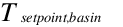 = Basin heater setpoint
temperature (oC)
= Basin heater setpoint
temperature (oC)
 = Outdoor air dry-bulb
temperature (oC)
= Outdoor air dry-bulb
temperature (oC)
 = Basin heater capacity
(W/K)
= Basin heater capacity
(W/K)
 = Run time fraction of DX
cooling coil
= Run time fraction of DX
cooling coil
The multimode DX coil uses 1 to 4 set of performance
specifications which all feed into the main DX coil model as
described above. The multimode DX coil may have 1 or 2
capacity stages and may have 1 enhanced dehumidification mode
in addition to its “normal” or base mode performance. Any mode
may specify that a portion of the total airflow is
bypassed.
Bypass Operation[LINK]
When a mode has coil bypass, the non-bypassed air flow
fraction is used to model the DX coil performance as described
above. Then the bypassed air stream is mixed with the
conditioned air stream and these conditions are place on the
coil outlet node.
Multi-Stage Operation[LINK]
Multi-stage control is modeled with the DX coil. If 2-stage
operation has been specified, stage 1 is assumed to operate
first and continue to operate if stage 2 is required. If
latent degradation is active, only one of the stages will be
degraded. If stage 1 operates for less than the full time
step, then latent degradation is applied. If stage 2 operates,
then stage 1 is running for the full time step and latent
degradation is applied only to the portion of the latent load
which is attributed to stage 2 operation.
Enhanced
Dehumidification Mode[LINK]
If enhanced dehumidification mode is available, this is
controlled by the parent object of the DX coil, such as
DXSystem:AirLoop. A dehumidification mode flag is passed to
the coil model which is used to select a different set of
performance specifications from a CoilPerformance:DX:Cooling
input object. Then the simulation of the DX coil proceeds as
described above including any bypass or multi-stage
operation.
Standard
Rating of Single-Speed DX Cooling Coils[LINK]
For small single-speed direct expansion (DX) cooling coils,
the industry standard ratings of Standard Rating Cooling
Capacity and Seasonal Energy Efficiency Ratio (SEER) are
calculated according to ANSI/AHRI Standard 210/240 (AHRI
2008). These ratings apply to unitary air conditioners and
air-source unitary heat pumps with air-cooled condensers with
standard rating cooling capacities under 19 kW (<65,000
Btu/hr). For larger DX cooling coils, the industry standard
ratings of Standard Rating Cooling Capacity, Energy Efficiency
Ratio (EER), and Integrated Energy Efficiency Ratio (IEER) are
calculated according to ANSI/AHRI Standard 340/360 (AHRI
2007). These ratings apply to unitary air conditioners and
air-source unitary heat pumps with standard rating cooling
capacities from 19 kW to below 73.2 kW (65,000 Btu/hr to
<250,000 Btu/hr).
For the Coil:Cooling:DX:SingleSpeed
object in EnergyPlus, these standard ratings are not direct
inputs to the model. However, these standard ratings can be
calculated using user-entered information for the Coil:Cooling:DX:SingleSpeed
object. Since users sometimes lump the performance of several
smaller DX cooling units into a single larger cooling coil
object for simulation purposes, EnergyPlus outputs the
Standard Rating Cooling Capacity, SEER, EER, and IEER
regardless of the magnitude of the standard rating cooling
capacity of the coil. It is up to the user to determine which
standard ratings are applicable to the cooling coil(s) they
are modeling. These standard rating values are provided in the
eplusout.eio output file (Ref. OutputDetailsAndExamples.pdf)
and also in the predefined tabular output reports
(Output:Table:SummaryReports object, Equipment Summary).
Currently, the standard ratings are only calculated and output
for single-speed DX cooling coils with air-cooled condensers.
If the single-speed DX coling coil is specified with an
evaporatively-cooled condenser, then no standard ratings are
output from EnergyPlus at this time.
Note: The standard ratings described in this section
require that the DX cooling coil model be evaluated at
specific operating conditions (i.e., specific wet-bulb
temperatures for air entering the cooling coil and dry-bulb
temperatures for air entering the air-cooled [outdoor]
condenser). If the cooling coil performance curves can not be
evaluated at the required test conditions, then a standard
rating value calculated at the curves limit will be output and
a warning message will written to eplusout.err. For example,
if the curve object (Curve:Biquadratic) for Total Cooling
Capacity Function of Temperature Curve has a minimum value of
21C for dry-bulb temperature entering the air-cooled condenser
coil, the IEER calculation requires that EERD be
calculated at 18.3C – so, this would result in IEER calculatd
at user specified curve limit as an output and a warning
message in the eplusout.err file.
The standard rating cooling capacity (AHRI 2007, AHRI 2008)
is calculated as follows:
where,
 = Standard Rating (Net)
Cooling Capacity (W)
= Standard Rating (Net)
Cooling Capacity (W)
 = Rated Total (Gross)
Cooling Capacity, user input (W)
= Rated Total (Gross)
Cooling Capacity, user input (W)
 = Total Cooling Capacity
Function of Temperature Curve evaluated with 19.44°C wet-bulb
temperature air entering the cooling coil and 35.0°C dry-bulb
temperature air entering the air-cooled (outdoor) condenser
(dimensionless)
= Total Cooling Capacity
Function of Temperature Curve evaluated with 19.44°C wet-bulb
temperature air entering the cooling coil and 35.0°C dry-bulb
temperature air entering the air-cooled (outdoor) condenser
(dimensionless)
 = Total Cooling Capacity
Function of Flow Fraction Curve evaluated at a flow fraction
of 1.0 (dimensionless)
= Total Cooling Capacity
Function of Flow Fraction Curve evaluated at a flow fraction
of 1.0 (dimensionless)
 = Rated Evaporator Fan
Power Per Volume Flow Rate, user input ( W/(m3/s)
)
= Rated Evaporator Fan
Power Per Volume Flow Rate, user input ( W/(m3/s)
)
 = Rated Air Volume Flow
Rate, user input (m3/s)
= Rated Air Volume Flow
Rate, user input (m3/s)
The Rated Evaporator Fan Power Per Volume Flow rate is a
user-entered value, with a default of 773.3
W/(m3/s)) if the user leaves this input field
blank. The default value is taken from ANSI/AHRI Standards
210/240 and 340/360 where it is defined for systems which do
not have a cooling coil fan furnished as part of the system
(e.g., a DX cooling coil mounted in the ductwork downstream of
a gas furnace where the furnace contains the fan used for air
distribution across the gas heating coil and the downstream DX
cooling coil). The test conditions in ANSI/AHRI Standards
210/240 and 340/360 vary the external static pressure (i.e.,
pressure drop associated with ductwork and other devices
external to the indoor fan/coil section) seen by the supply
air fan based on the standard rating cooling capacity. Note,
however, that external static pressure in actual installations
is typically much higher. Further details regarding indoor fan
power per volume flow rate can be found in Walker and Lutz
(2005) and Walker (2007), including differences between
Permanent Split Capacitor (PSC) and Brushless Permanent Magnet
(BPM) fan motors. Especially at the low external static
pressures defined in the ANSI/AHRI Standards, BPM motors
(e.g., Electronically Commutated Motors (ECMs)) can draw
significantly less power (e.g., 50-75% less) than PSC
motors.
The seasonal energy efficiency ratio (SEER) is calculated
as follows:


where,
PLF0.5~~ =Part Load Fraction
Correlation Curve evaluated at a part load ratio (PLR) of 0.5
(dimensionless)
EERTestB~~ =Energy efficiency ratio
with 19.44°C wet-bulb temperature air entering the cooling
coil, 27.78°C dry-bulb temperature air entering the air-cooled
(outdoor) condenser, and rated air volume flow through the
cooling coil (W/W)
 = Net total cooling
capacity with 19.44°C wet-bulb temperature air entering the
cooling coil, 27.78°C dry-bulb temperature air entering the
air-cooled (outdoor) condenser, and rated air volume flow
through the cooling coil (W)
= Net total cooling
capacity with 19.44°C wet-bulb temperature air entering the
cooling coil, 27.78°C dry-bulb temperature air entering the
air-cooled (outdoor) condenser, and rated air volume flow
through the cooling coil (W)
 = Total Cooling Capacity
Function of Temperature Curve evaluated with 19.44°C wet-bulb
temperature air entering the cooling coil and 27.78°C dry-bulb
temperature air entering the air-cooled (outdoor) condenser
(dimensionless)
= Total Cooling Capacity
Function of Temperature Curve evaluated with 19.44°C wet-bulb
temperature air entering the cooling coil and 27.78°C dry-bulb
temperature air entering the air-cooled (outdoor) condenser
(dimensionless)
 = Total electric power
(compressors, condenser fans and evaporator fan) with 19.44°C
wet-bulb temperature air entering the cooling coil, 27.78°C
dry-bulb temperature air entering the air-cooled (outdoor)
condenser, and rated air volume flow through the cooling coil
(W)
= Total electric power
(compressors, condenser fans and evaporator fan) with 19.44°C
wet-bulb temperature air entering the cooling coil, 27.78°C
dry-bulb temperature air entering the air-cooled (outdoor)
condenser, and rated air volume flow through the cooling coil
(W)
 = Coefficient of
Performance at Rated Conditions, user input (W/W)
= Coefficient of
Performance at Rated Conditions, user input (W/W)
 = Energy Input Ratio
Function of Temperature Curve evaluated with 19.44°C wet-bulb
temperature air entering the cooling coil and 27.78°C dry-bulb
temperature air entering the air-cooled (outdoor) condenser
(dimensionless)
= Energy Input Ratio
Function of Temperature Curve evaluated with 19.44°C wet-bulb
temperature air entering the cooling coil and 27.78°C dry-bulb
temperature air entering the air-cooled (outdoor) condenser
(dimensionless)
 = Energy Input Ratio
Function of Flow Fraction Curve evaluated at a flow fraction
of 1.0 (dimensionless).
= Energy Input Ratio
Function of Flow Fraction Curve evaluated at a flow fraction
of 1.0 (dimensionless).
Energy Efficiency Ratio (EER) is another standard rating
(AHRI 2007), and it is defined as the ratio of the total
cooling capacity to the total power input at any given set of
rating conditions, expressed in W/W (or Btu/W-h). For this
class of air-cooled DX cooling coils, EER is calculated at
rated test conditions as follows:
where,
EER = Energy Efficiency Ratio (W/W)
 = Total electric power
(compressors, condenser fans and evaporator fan) with 19.44°C
wet-bulb temperature air entering the cooling coil, 35.0°C
dry-bulb temperature air entering the air-cooled (outdoor)
condenser, and air flow rate across the evaporator at the
Rated Air Volume Flow Rate (W).
= Total electric power
(compressors, condenser fans and evaporator fan) with 19.44°C
wet-bulb temperature air entering the cooling coil, 35.0°C
dry-bulb temperature air entering the air-cooled (outdoor)
condenser, and air flow rate across the evaporator at the
Rated Air Volume Flow Rate (W).
 = Total Cooling Capacity
Function of Temperature Curve evaluated with 19.44°C wet-bulb
temperature air entering the cooling coil and 35.0°C dry-bulb
temperature air entering the air-cooled (outdoor) condenser
(dimensionless)
= Total Cooling Capacity
Function of Temperature Curve evaluated with 19.44°C wet-bulb
temperature air entering the cooling coil and 35.0°C dry-bulb
temperature air entering the air-cooled (outdoor) condenser
(dimensionless)
 = Energy Input Ratio
Function of Temperature Curve evaluated with 19.44°C wet-bulb
temperature air entering the cooling coil and 35.0°C dry-bulb
temperature air entering the air-cooled (outdoor) condenser
(dimensionless)
= Energy Input Ratio
Function of Temperature Curve evaluated with 19.44°C wet-bulb
temperature air entering the cooling coil and 35.0°C dry-bulb
temperature air entering the air-cooled (outdoor) condenser
(dimensionless)
The Integrated Energy Efficiency Ratio (IEER) is intended
to be a measure of merit for the cooling coil’s part-load
efficiency. IEER replaced Integrated Part-Load Value (IPLV) as
the part-load performance metric in Std. 340/360 as of January
1, 2010. Full details regarding the IEER calculation are
available in ANSI/AHRI Std. 340/360 (AHRI 2007). A summary of
the IEER calculations made by EnergyPlus for single-speed
air-cooled DX cooling coils is provided below:
where,
 =EER at 100% net
capacity at AHRI standard rating conditions (same as EER
calculation shown above)
=EER at 100% net
capacity at AHRI standard rating conditions (same as EER
calculation shown above)
 =EER at 75% net
capacity and reduced outdoor air temperature
=EER at 75% net
capacity and reduced outdoor air temperature
 =EER at 50% net
capacity and reduced outdoor air temperature
=EER at 50% net
capacity and reduced outdoor air temperature
 =EER at 25% net
capacity and reduced outdoor air temperature
=EER at 25% net
capacity and reduced outdoor air temperature
where,
 =Net total cooling
capacity with 19.44°C wet-bulb temperature air entering the
cooling coil rated air volume flow through the cooling coil
(W). The dry-bulb temperature of air entering the air-cooled
condenser varies (B = 27.5°C, C = 20.0°C, D = 18.3°C).
=Net total cooling
capacity with 19.44°C wet-bulb temperature air entering the
cooling coil rated air volume flow through the cooling coil
(W). The dry-bulb temperature of air entering the air-cooled
condenser varies (B = 27.5°C, C = 20.0°C, D = 18.3°C).
 = Total electric power
(compressors, condenser fans and evaporator fan) with 19.44°C
wet-bulb temperature air entering the cooling coil and air
flow rate across the evaporator at the Rated Air Volume Flow
Rate (W). The dry-bulb temperature of air entering the
air-cooled condenser varies (B = 27.5°C, C = 20.0°C, D =
18.3°C).
= Total electric power
(compressors, condenser fans and evaporator fan) with 19.44°C
wet-bulb temperature air entering the cooling coil and air
flow rate across the evaporator at the Rated Air Volume Flow
Rate (W). The dry-bulb temperature of air entering the
air-cooled condenser varies (B = 27.5°C, C = 20.0°C, D =
18.3°C). = Electric power of
the compressor and condenser fan at the various part-load
ratios, with 19.44°C wet-bulb temperature air entering the
cooling coil and rated supply air volume flow rate (W). The
dry-bulb temperature of air entering the air-cooled condenser
varies per the part-load ratio (B = 27.5°C, C = 20.0°C, D =
18.3°C).
= Electric power of
the compressor and condenser fan at the various part-load
ratios, with 19.44°C wet-bulb temperature air entering the
cooling coil and rated supply air volume flow rate (W). The
dry-bulb temperature of air entering the air-cooled condenser
varies per the part-load ratio (B = 27.5°C, C = 20.0°C, D =
18.3°C).
 = Energy Input Ratio
Function of Temperature Curve evaluated with 19.44°C wet-bulb
temperature air entering the cooling coil and dry-bulb
temperature of air entering the air-cooled condenser
corresponding to the reduced part-load ratio (B = 27.5°C, C =
20.0°C, D = 18.3°C) (dimensionless).
= Energy Input Ratio
Function of Temperature Curve evaluated with 19.44°C wet-bulb
temperature air entering the cooling coil and dry-bulb
temperature of air entering the air-cooled condenser
corresponding to the reduced part-load ratio (B = 27.5°C, C =
20.0°C, D = 18.3°C) (dimensionless).
 = degradation coefficient
to account for cycling of the compressor = 1.13 –
0.13LF.
= degradation coefficient
to account for cycling of the compressor = 1.13 –
0.13LF.
 = fractional “on” time at
the desired load point
= fractional “on” time at
the desired load point
The load factor (LF) is the fractional “on” time
for the desired reduced load points (75%, 50%, or 25%)
calculated from the following equation:
where,
 =
Part-load operating points, i.e., 75% (B), 50% (C), 25%
(D)
=
Part-load operating points, i.e., 75% (B), 50% (C), 25%
(D)
The calculations for
QTotal,Net,PartLoad and
PowerTotal,PartLoad are calculated in
nearly the same way as QTotal,Net,TestB
and PowerTotal,TestB are calculated for
SEER (defined above). The only difference is that these
cooling capacity and power values, used for calculating
EERB/EERC/EERD for IEER, are
calculated for a series of dry-bulb temperatures of air
entering the air-cooled condenser (B = 27.5°C, C = 20.0°C, D =
18.3°C) and part-load performance degradiation correction is
also applied to the condensing unit electric power
calculation.


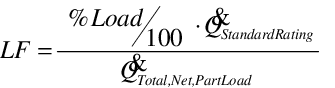

Basin Heater For
Two-Stage DX Coil[LINK]
Basin heater for the object Coil:Cooling:DX:TwoStageWithHumidityControlMode
operates in the same manner as for Coil:Cooling:DX:SingleSpeed.
Refer to the “Basin Heater For Single-Speed DX Coil”
description above.
If the number of capacity stages is equal to 1 and the
CondenserType for that stage is EvapCooled, then the basin
heater power is calculated for (1 - RunTimeFractionStage1) of
DX coil.
If the number of capacity stages is greater than 1,
then
If the CondenserType for stage 1 is EvapCooled, then the
basin heater power is calculated for (1 -
RunTimeFractionStage1) of DX coil
Elseif the CondenserType for stage 2 is EvapCooled, then
the basin heater power is calculated for (1 -
RunTimeFractionStage2) of DX coil
AHRI 2008. ANSI/AHRI Standard 210/240: 2008 Standard for
Performance Rating of Unitary Air-Conditioning &
Air-Source Heat Pump Equipment. Arlington, VA:
Air-Conditioning, Heating, and Refrigeration Institute.
AHRI 2007. ANSI/AHRI Standard 340/360: 2007 Standard for
Performance Rating of Commercial and Industrial Unitary
Air-Conditioning and Heat Pump Equipment. Arlington, VA:
Air-Conditioning, Heating, and Refrigeration Institute.
ASHRAE. 1993. HVAC2 Toolkit: A Toolkit for Secondary HVAC
System Energy Calculation. Atlanta: American Society of
Heating, Refrigerating and Air-Conditioning Engineers,
Inc.
Carrier, W.H., R.E. Cherne, W.A. Grant, and W.H. Roberts.
1959. Modern air conditioning, heating and
ventilating, 3d ed. New York: Pitman Publishing
Corporation.
Henderson, H.I. Jr., K. Rengarajan, and D.B. Shirey III.
1992. The impact of comfort control on air conditioner energy
use in humid climates. ASHRAE Transactions 98(2):
104-113.
Henderson, H.I. Jr. and K. Rengarajan. 1996. A Model to
Predict the Latent Capacity of Air Conditioners and Heat Pumps
at Part-Load Conditions with Constant Fan Operation.
ASHRAE Transactions 102(2): 266-274.
Henderson, H. 1998. The impact of part load air conditioner
operation on dehumidification performance: Validating a latent
capacity degradation model. Presented at ASHRAE’s IAQ &
Energy ’98 conference. New Orleans, LA. October.
Henderson, H. and D. Shirey. 2003. Understanding the
Dehumidification Performance of Air-Conditioning Equipment at
Part-Load Conditions. Paper presented at Joint CIBSE/ASHRAE
Conference, Building
Sustainability, Value and Profit. September. Edinburgh,
Scotland.
Walker, I.S. and Lutz, J.D. 2005. Laboratory Evaluation of
Residential Furnace Blower Performance. Berekely, CA: Lawrence
Berkeley National Laboratory, Report LBNL 58752.
Walker, I.S. 2007. Comparing Residential Furnace Blowers
for Rating and Installed Performance. Berkeley, CA: Lawrence
Berkeley National Laboratory, Environmental Energy
Technologies Division Report LBNL 62344.
Multi-Speed
Electric DX Air Cooling Coil[LINK]
This model (object name Coil:Cooling:DX:MultiSpeed)
simulates the performance of an air-to-air direct expansion
(DX) cooling system. The main difference compared to the other
cooling coil models, such as Coil:Cooling:DX:SingleSpeed,
is that this cooling coil allows modeling of two to four
discrete compressor speeds. Each speed has a set of
corresponding performance information at rated conditions
along with curve fits for variations in total capacity, SHR,
energy input ratio and part-load fraction to determine the
performance of the unit at part-load conditions (DOE 1982).
The full load supply airflow rate is dependent on the speed
number and provided by its parent object (Ref.
AirLoopHVAC:UnitaryHeatPump:AirToAir:MultiSpeed). The
part-load impact on coil energy use is automatically applied
to the lowest speed. A choice is provided to determine whether
part-load impacts on coil energy use are applied when the coil
is operating at speeds greater than speed 1.
This model simulates the thermal performance of the indoor
DX cooling coil, and the power consumption of the outdoor unit
(multispeed compressor, fans, and crankcase heaters). The
performance of the indoor supply air fan varies widely from
system to system depending on control strategy (e.g., constant
fan vs. AUTO fan), fan type, fan motor efficiency and pressure
losses through the air distribution system. Therefore, this DX
system model does not account for the thermal effects or
electric power consumption of the indoor supply air fan.
EnergyPlus contains separate models for simulating the
performance of various indoor fan configurations, and these
models can be easily linked with the DX system model described
here to simulate the entire DX system being considered. For
the time being, this coil model can only be called by the
parent object AirLoopHVAC:UnitaryHeatPump:AirToAir:MultiSpeed.
When the model determines performance at Speed 1 (the
lowest speed) or cycling between OFF and Speed 1, its
performance is almost the same as the performance for the Coil:Cooling:DX:SingleSpeed
model. However, the outlet conditions are calculated slightly
differently. Therefore, the Coil:Cooling:DX:SingleSpeed
model may be considered as a subset of the model described
here. When the multispeed coil model determines performance at
higher speeds (above 1), the model linearly interpolates the
performance at two consecutive speeds (n-1 and n) as needed to
meet the cooling load, with the fraction of time at each speed
established by the speed ratio.
The model inputs are also very similar to the inputs of the
Coil:Cooling:DX:SingleSpeed
object. The main difference is that this multispeed model
requires a set of fields at each speed, such as rated
capacity, rated SHR, rated COP, two capacity modifiers, two
energy input ratio modifiers, part-load correction, and latent
degradation inputs. The inputs also include waste heat
fraction at the rated conditions and modifier as a function of
temperature to calculate recoverable waste heat for heat
recovery, which are not available in the similar Coil:Cooling:DX:SingleSpeed
object
Speed 1 Operation[LINK]
The calculation procedures in this model, including defrost
and crankcase heater, are indentical to the Coil:Heating:DX:SingleSpeed
object (Ref: Coil:Heating:DX:SingleSpeed) with one exception:
outlet node condition calculation when the supply air fan
operates continuously (i.e., supply air fan operating mode
schedule value is not equal to 0; Ref.
AirLoopHVAC:UnitaryHeatPump:AirToAir:MultiSpeed).
The following procedure provides the detailed description
of the exception.
- Total delivered cooling capacity
The total delivered cooling capacity for speed 1 operating
at the cycling ratio needed to meet the requested cooling load
is:
where,
Qcoil,cyclingl= delivered total cooling
capacity for Speed 1 operating at a specific cycling ratio
[W]
 = air mass flow rate
through cooling coil at Speed 1 as set by the parent object
[kg/s]
= air mass flow rate
through cooling coil at Speed 1 as set by the parent object
[kg/s]
houtlet,full= specific enthalpy of the
coil outlet air during full-load operation at Speed 1 (no
cycling) [J/kg]
hinlet= specific enthalpy of the coil inlet
air [J/kg]
CycRatio= cycling ratio at Speed 1, ratio of
requested heating load to the full-load capacity of the coil
at Speed 1 [dimensionless]
It is assumed that the coil provides no cooling capacity
when the coil is OFF, even if the supply air fan continues to
operate.
- Outlet air specific enthalpy
The average specific enthalpy of the coil outlet air is
then calculated based on the total delivered cooling capacity
and the average air mass flow rate entering the coil:
where
houtlet,average= averaged specific enthalpy at
the coil outlet [J/kg]
hinlet= specific enthalpy at the coil inlet
[J/kg]
Qcoil,cycling= total capacity at full load
[W]
 = mass flow rate at the
inlet to the coil as established by the parent object (Ref. AirLoopHVAC:UnitaryHeatPump:AirToAir:MultiSpeed,
Mass Flow Rate Calculation). This flow rate is the average
value determined by the parent object, accounting for the
specified flow rate when the cooling coil is ON and the
specified flow rate when the cooling coil is OFF for the time
step being simulated.
= mass flow rate at the
inlet to the coil as established by the parent object (Ref. AirLoopHVAC:UnitaryHeatPump:AirToAir:MultiSpeed,
Mass Flow Rate Calculation). This flow rate is the average
value determined by the parent object, accounting for the
specified flow rate when the cooling coil is ON and the
specified flow rate when the cooling coil is OFF for the time
step being simulated.
The minimum humidity ratio (HRmin ) is based on
humidity ratios between inlet and full load outlet as:
HRmin = Minimum(HRinlet,
HRfull)
where
HRinlet= Humidity ratio at the inlet [kg/kg]
HRfull= Full load humidity ratio at the outlet
[kg/kg]
The coil sensible capacity may be calculated as:
where
Qcoil,sens= delivered sensible cooling capacity
[W]
houtlet,full= full load specific enthalpy at the
coil outlet as a function of outlet dry-bulb temperature at
the full load, and the minimum humidity ratio [J/kg]
hinlet= specific enthalpy at the coil inlet
[J/kg]
The latent capacity is the difference between total and
sensible capacities
where
Qcoil,latent= delivered latent cooling capacity
[W]
- Average outlet air humidity ratio
The averaged outlet HR can be calculated as:
where
λ= heat of vaporization as a function of HRmin
and
CycRatio*Toutlet,full+(1-CycRatio)*Tinlet~~[J/kg]
- Average outlet air temperature
Using the above averaged outlet humidity ratio and specific
enthalpy, the averaged outlet temperature can be calculated
using the psych function of PsyTdbFnHW.
The main reason using the above approach is that outlet
conditions are calculated in the same way in low and high
speed operation.
The crankcase heater defined for this DX cooling coil is
enabled during the time that the compressor is not running for
either heating or cooling. The crankcase heater power use from
either heating or cooling is reported in the heating coil
(Coil:Heating:DX:MultiSpeed).
Higher Speed Operation[LINK]
This section describes how higher speed operation is
simulated. When the required sensible load is less than the
full load sensible capacity at Speed n (Speed Number > 1),
the following calculations are performed:
- Bypass factor at Speed n-1 and Speed n
where
BypassFactori= bypass factor at actual flow rate
conditions at Speed i [dimensionless]
RatedBypassFactori= bypass factor at the rated
conditions at Speed i [dimensionless]
RatedFowRatei= air mass flow rate at the rated
conditions at Speed i [kg/s]
ActualFowRatei= actual air mass flow rate at
Speed i [kg/s]
i= Speed n or Speed n-1
The bypass factor at Speed n is a function of the bypass
factor at the rated conditions, rated airflow rate, and actual
flow rate at Speed n. The calculation is performed by a
function, called AdjustCBF in the DXCoil module.
- Total capacity at Speed n-1 and Speed n


where
TotCapi= total cooling capacity at given
temperatures and flow rates at Speed i [w]
RatedCapi= cooling capacity at the rated
conditions at Speed i [W]
TotCapTempModFaci= total cooling capacity
modifier as a function of indoor web-bulb temperature and
outdoor air dry-bulb temperature at Speed i
TotCapFlowModFaci= total cooling capacity
modifier as a function of the ratio of the actual flow rate
across the cooling coil to the rated airflow rate at Speed
i
i= Speed n or Speed n-1
The calculation is performed by a subroutine, called
CalcTotCapSHR in the DXCoil module.
- EIR at Speed n-1 and Speed n
where
EIRi= Energy input ratio at given temperatures
and flow rates at Speed i [w]
RatedEIRi= Energy input ratio at the rated
conditions at Speed i [W]
EIRTempModFaci= Energy input ratio modifier as a
function of indoor and outdoor air dry-bulb temperature at
Speed i
EIRFlowModFaci= Energy input ratio modifier as a
function of ratio of the actual flow rate across the heating
coil to the rated airflow rate at Speed i
i= n or n-1
- Full load outlet conditions at Speed n-1 and Speed n
The calculation procedure of full load outlet conditions at
Speed n-1 and Speed n is the same as the calculation procedure
used in the Coil:Cooling:DX:SingleSpeed
model (Ref. Coil:Cooling:DX:SingleSpeed). The difference is
that the outlet conditions at Speed n-1 are calculated based
on the total cooling capacity and mass flow rate at Speed n-1,
while the outlet conditions at Speed n are calculated based on
the total cooling capacity and mass flow rate at Speed n.
- Effective total cooling capacity
where
 = delivered sensible
cooling capacity at a given speed ratio between two
consecutive speeds [W]
= delivered sensible
cooling capacity at a given speed ratio between two
consecutive speeds [W]
 = air mass flow rate
through cooling coil at Speed n as set by the parent object
[kg/s]
= air mass flow rate
through cooling coil at Speed n as set by the parent object
[kg/s]
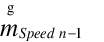 = air mass flow rate
through cooling coil at Speed 1 as set by the parent object
[kg/s]
= air mass flow rate
through cooling coil at Speed 1 as set by the parent object
[kg/s]
hinlet= specific enthalpy at the coil inlet
[J/kg]
houtlet~,full_Speed n~= full load specific
enthalpy at the coil outlet at Speed n [J/kg]
houtlet~,full_Speed n-1~= full load specific
enthalpy at the coil outlet at Speed n-1 [J/kg]
- Average outlet air specific enthalpy
where
houtlet,average= averaged specific enthalpy at
the coil outlet [J/kg]
hinlet= specific enthalpy at the coil inlet
[J/kg]
 = mass flow rate at the
inlet to the coil as established by the parent object (Ref. AirLoopHVAC:UnitaryHeatPump:AirToAir:MultiSpeed,
Mass Flow Rate Calculation). This flow rate is the average
value determined by the parent object, accounting for the
specified flow rate when the heating coil is at Speed n and
the specified flow rate when the heating coil is at Speed n-1
for the time step being simulated.
= mass flow rate at the
inlet to the coil as established by the parent object (Ref. AirLoopHVAC:UnitaryHeatPump:AirToAir:MultiSpeed,
Mass Flow Rate Calculation). This flow rate is the average
value determined by the parent object, accounting for the
specified flow rate when the heating coil is at Speed n and
the specified flow rate when the heating coil is at Speed n-1
for the time step being simulated.
- Effective sensible cooling capacity
The minimum humidity ratio (HRmin ) is
calculated as
HRmin = Minimum[HRinlet,
(SpeedRatio)HRfull,n+(1.0-SpeedRatio)HRfull,n-1)
The effective sensible cooling capacity is expressed
as:
where
Qcoil,sens= effective sensible cooling capacity
[W]
houtlet~,full_Speed n~ = full load specific
enthalpy at the coil outlet at Speed n as a function of outlet
dry-bulb temperature at the full load, and the minimum
humidity ratio [J/kg]
houtlet~,full_Speed n-1~ = full load specific
enthalpy at the coil outlet at Speed n-1 as a function of
outlet dry-bulb temperature at the full load, and the minimum
humidity ratio [J/kg]
hinlet= specific enthalpy at the coil inlet
[J/kg]
- Aaverage outlet air humidity ratio and temperature
The effective latent cooling capacity is the difference
between the total and sensible capacity:
Qcoil,latent= effective latent cooling capacity
[W]
The average outlet air HR can be calculated as:
where
λ= heat of vaporization as a function of HRmin
and
SpeedRatio*Toutlet,n+(1-SpeedRatio)*Toutlet,n-1[J/kg]
At the given averaged outlet humidity ratio and specific
enthalpy, the averaged outlet temperature can be calculated
using the psych function of PsyTdbFnHW.
- Calculate combined energy input
When the input for the field ‘Apply Part Load Fraction to
Speeds Greater than 1’ is No in the object (equivalent to a
single compressor), the combined energy output is calculated
as follows:
 When the input for the
field ‘Apply Part Load Fraction to Speeds Greater than 1’ is
Yes in the object (equivalent to multiple compressors), the
combined energy output is calculated as follows:
When the input for the
field ‘Apply Part Load Fraction to Speeds Greater than 1’ is
Yes in the object (equivalent to multiple compressors), the
combined energy output is calculated as follows:
where
CoolingPower= Power used in Watt
RTF= Run time fraction at Speed n
When the supply fan operation mode is
ContinuousFanWithCyclingCompressorand the input of the Apply
Latent Degradation to Speeds Greater than 1 is Yes, the latent
degradation is included at Speed n. The calculation procedure
is the same as one in the Coil:Cooling:DX:SingleSpeed
object. The difference is that the rated values and run time
fraction at Speed n are used. The adjusted SHR is used to
calculate full load outlet conditions at Speed n.
It is expected to have less latent degradation at Speed n
than Speed 1. Therefore, smaller values of the latent
degradation inputs at Speed n than those at Speed 1 are
recommended.
There is no power need at higher speed operation.
Waste heat calculation[LINK]
The waste heat generated by this coil object is calculated
as:
where
Fraction= rated waste heat fraction of the energy input
TempModifer= waste heat modifier as a function of indoor
and outdoor air dry-bulb temperature
Basin Heater For
Multi-Speed DX Coil[LINK]
Basin heater for the object Coil:Cooling:DX:MultiSpeed
operates in the same manner as for Coil:Cooling:DX:SingleSpeed.
Refer to the Basin Heater For Single-Speed DX Coil description
above.
Standard
Rating of Multi-Speed DX Cooling Coils[LINK]
For multi-speed direct expansion cooling coils, the
industry standard ratings of Standard Rating Seasonal Energy
Efficiency Ratio (SEER) are calculated according to ANSI/AHRI
Standard 210/240 (AHRI 2008). These standard ratings can be
calculated using the user-entered information for the Coil:Cooling:DX:MultiSpeed
object. According to Standard 210/240, the Standard Rating
SEER applies to air-to-air unitary heat pumps and air
conditions with rated cooling capacities under 19,000 Watts
(<65,000 Btu/h). The Cooling Mode Test Conditions for Units
Having two-capacity Compressor standard tests A2,
B2, B1, and F1 are also
provided in Table 49. Cooling Mode Test Conditions for Units
Having a Two-Capacity Compressor. The equations required to
calculate the net cooling capacity and SEER value are
described next.
Standard Rating
Cooling Capacity[LINK]
The standard net cooling capacity of multi-speed DX cooling
coil is reported at the maximum speed and full load A2 test
condition only. The Standard Rating (Net) Cooling Capacity
calculation is the same as single speed DX cooling coil
procedure when calculated at maximum speed. The procedure for
calculating the Standard Rating Cooling Capacity is given
by:
where,
 =total standard
(net) cooling capacity (W) of the
air-conditioning or heat pump equipment in cooling mode
determined from ANSI/AHRI Standard 210/240 and A2 test
conditions shown in Table 49. The standard cooling test
conditions for air-cooled condenser are: indoor coil entering
air dry-bulb and wet-bulb temperatures 26.7°C/19.4°C and
outdoor coil entering air dry-bulb and wet-bulb temperatures
35.0°C/23.9°C.
=total standard
(net) cooling capacity (W) of the
air-conditioning or heat pump equipment in cooling mode
determined from ANSI/AHRI Standard 210/240 and A2 test
conditions shown in Table 49. The standard cooling test
conditions for air-cooled condenser are: indoor coil entering
air dry-bulb and wet-bulb temperatures 26.7°C/19.4°C and
outdoor coil entering air dry-bulb and wet-bulb temperatures
35.0°C/23.9°C.
 =total standard cooling
capacity (W) of the air-conditioning or heat pump equipment
determined from ANSI/AHRI Standard 210/240 and A2 test
conditions shown in Table 49. The standard cooling test
conditions for air-cooled are: indoor coil entering air
dry-bulb and wet-bulb temperatures 26.7°C/19.4°C and outdoor
coil entering air dry-bulb and wet-bulb temperatures
35.0°C/23.9°C.
=total standard cooling
capacity (W) of the air-conditioning or heat pump equipment
determined from ANSI/AHRI Standard 210/240 and A2 test
conditions shown in Table 49. The standard cooling test
conditions for air-cooled are: indoor coil entering air
dry-bulb and wet-bulb temperatures 26.7°C/19.4°C and outdoor
coil entering air dry-bulb and wet-bulb temperatures
35.0°C/23.9°C.
 = Rated total cooling
capacity at maximum speed, user input (W)
= Rated total cooling
capacity at maximum speed, user input (W)
 = User-specified
bi-quadratic curve evaluated at the indoor coil entering air
wet-bulb temperature (19.4°C) and outdoor coil entering air
dry-bulb temperature (35.0°C) for air-cooled condenser per A2
test condition as specified in Table 49, (dimensionless).
= User-specified
bi-quadratic curve evaluated at the indoor coil entering air
wet-bulb temperature (19.4°C) and outdoor coil entering air
dry-bulb temperature (35.0°C) for air-cooled condenser per A2
test condition as specified in Table 49, (dimensionless).
 = User-specified
quadratic or cubic curve modifying the total cooling capacity
as function of flow fraction, (dimensionless). This curve is
evaluated at a flow fraction of 1.0.
= User-specified
quadratic or cubic curve modifying the total cooling capacity
as function of flow fraction, (dimensionless). This curve is
evaluated at a flow fraction of 1.0.
 = Supply air fan power at
rated conditions at high (maximum) compressor speed, (W).
= Supply air fan power at
rated conditions at high (maximum) compressor speed, (W).
 = Rated Air Volume Flow
Rate at high (maximum) compressor speed, user input
(m3/s)
= Rated Air Volume Flow
Rate at high (maximum) compressor speed, user input
(m3/s)
 = The Rated Indoor Coil
Fan Power Per Volume Flow rate is a user-entered value, with a
default of 775 W/(m3/s)) if the user leaves this
input field blank. The default value is taken from ANSI/ASHRAE
Standard 210/240 -2008 where it is defined for systems which
do not have an indoor coil fan furnished as part of the
system. See the description given below how this value is
calculated. User input ( W/(m3/s)).
= The Rated Indoor Coil
Fan Power Per Volume Flow rate is a user-entered value, with a
default of 775 W/(m3/s)) if the user leaves this
input field blank. The default value is taken from ANSI/ASHRAE
Standard 210/240 -2008 where it is defined for systems which
do not have an indoor coil fan furnished as part of the
system. See the description given below how this value is
calculated. User input ( W/(m3/s)).
The Rated Evaporator (Indoor Coil) Fan Power Per Volume
Flow rate is a user-entered value, with a default of 773.3
W/(m3/s)) if the user leaves this input field
blank. The default value is taken from ANSI/ASHRAE Standard
210/240-2008 where it is defined for systems which do not have
an Indoor Coil (Evaporator) fan furnished as part of the
system. The test conditions in ANSI/AHRI Standard 210/240 vary
the external static pressure (i.e., pressure drop associated
with ductwork and other devices external to the indoor
fan/coil section) seen by the supply air fan based on the
standard rating cooling capacity.
Seasonal
Energy Efficiency Ratio (SEER) for Multi-Speed DX Coil[LINK]
The SEER value for multi-speed compressor air conditioner
or air-to-air heat pumps per AHRI/ANSI Std. 210/240 – 2008 is
calculated as follows:
For multi-speed compressor the SEER value is weighted
average performance at different outdoor air temperature bins.
The eight outdoor air temperature bins and the corresponding
weight are provided in Table 50. Distribution of Fractional
Hours with in Cooling Season Temperature Bins.
Where,
qc(Tj)/N = = the ratio of
space cooling capacity provided by the unit during periods of
the space cooling season when the outdoor temperature fell
within the range represented by bin temperature
Tj to the total number of hours in the
cooling season (N), (W)
ec(Tj)/N = the ratio of the
electrical energy consumed by the unit during periods of the
space cooling season when the outdoor temperature fell within
the range represented by bin temperature Tj to the total
number of hours in the cooling season (N), W.
j = the bin number, dimensionless. For cooling
season j ranges from 1 to 8.
Tj= outdoor air bin temperature, °C.
Outdoor temperatures are “binned” such that calculations are
only performed based one temperature within the bin. Bins of
2.8 °C with 8 cooling season bin temperatures being 19.44°C,
22.22°C, 25.0°C, 27.78°C, 30.56°C, 33.33°C, 36.11°C,
38.89°C.
The steady-state cooling capacity delivered and the
electric power inputs when the DX coil is operating at minimum
compressor speed (k=1), and outdoor air temperature
Tj, are determined by linear interpolation
using the values of B1 and F1 tests as follows:
The steady-state cooling capacities and electric power
inputs at the minimum speed and test condition
B1~~and F1 are
calculated from the minimum (low) speed performance curves as
follows:
Where,
 =rated total cooling
capacity at minimum compressor speed specified by users,
(W)
=rated total cooling
capacity at minimum compressor speed specified by users,
(W)
 =rated gross COP at
minimum compressor speed specified by users, (-)
=rated gross COP at
minimum compressor speed specified by users, (-)
 =cooling capacities
modifier curve for temperature at minimum compressor speed and
B1 test condition, (-)
=cooling capacities
modifier curve for temperature at minimum compressor speed and
B1 test condition, (-)
 =cooling capacities
modifier curve for flow fraction at minimum compressor speed
and B1 test condition, (-)
=cooling capacities
modifier curve for flow fraction at minimum compressor speed
and B1 test condition, (-)
 =EIR modifier curve for
temperature at minimum compressor speed and B1 test condition,
(-)
=EIR modifier curve for
temperature at minimum compressor speed and B1 test condition,
(-)
 =EIR modifier curve for
flow fraction at minimum compressor speed and B1 test
condition, (-)
=EIR modifier curve for
flow fraction at minimum compressor speed and B1 test
condition, (-)
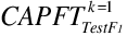 =cooling capacities
modifier curve for temperature at minimum compressor speed and
F1 test condition, (-)
=cooling capacities
modifier curve for temperature at minimum compressor speed and
F1 test condition, (-)
 =cooling capacities
modifier curve for flow fraction at minimum compressor speed
and F1 test condition, (-)
=cooling capacities
modifier curve for flow fraction at minimum compressor speed
and F1 test condition, (-)
 =EIR modifier curve for
temperature at minimum compressor speed and F1 test condition,
(-)
=EIR modifier curve for
temperature at minimum compressor speed and F1 test condition,
(-)
 =EIR modifier curve for
flow fraction at minimum compressor speed and F1 test
condition, (-)
=EIR modifier curve for
flow fraction at minimum compressor speed and F1 test
condition, (-)
 =the rated supply air fan
power when the unit is operating at minimum compressor speed,
(W)
=the rated supply air fan
power when the unit is operating at minimum compressor speed,
(W)
 =rated cooling supply air
volume flow rate at minimum compressor speed specified by
users, (-)
=rated cooling supply air
volume flow rate at minimum compressor speed specified by
users, (-)
 =the rated Indoor Coil
fan power per volume flow rate at low (minimum) compressor
speed specified value by the user, (W/(m3/s))
=the rated Indoor Coil
fan power per volume flow rate at low (minimum) compressor
speed specified value by the user, (W/(m3/s))
The steady-state cooling capacity delivered and the
electric power inputs when the DX cooling coil is operating at
maximum (high) compressor speed (k=2), and outdoor
air temperature Tj, are determined as
follows:
The steady-state cooling capacities and electric power
input at the maximum speed and test condition
A2 and B2 are
determined from the maximum (high) speed performance curves as
follows:


Where,
 = rated total cooling
capacity at maximum (high) compressor speed specified by
users, (W)
= rated total cooling
capacity at maximum (high) compressor speed specified by
users, (W)
 = rated gross COP at
maximum (high) compressor speed specified by users, (-)
= rated gross COP at
maximum (high) compressor speed specified by users, (-)
 = cooling capacity
modifier curve for temperature at maximum (high) compressor
speed and A2 test condition, (-)
= cooling capacity
modifier curve for temperature at maximum (high) compressor
speed and A2 test condition, (-)
 =cooling capacity
modifier curve for flow fraction at maximum (high) compressor
speed and A2 test condition, (-)
=cooling capacity
modifier curve for flow fraction at maximum (high) compressor
speed and A2 test condition, (-)
 = EIR modifier curve for
temperature at maximum (high) compressor speed and
A2 test condition, (-)
= EIR modifier curve for
temperature at maximum (high) compressor speed and
A2 test condition, (-)
 = EIR modifier curve for
flow fraction at maximum (high) compressor speed and
A2 test condition, (-)
= EIR modifier curve for
flow fraction at maximum (high) compressor speed and
A2 test condition, (-)
 = cooling capacity
modifier curve for temperature at maximum (high) compressor
speed and B2 test condition, (-)
= cooling capacity
modifier curve for temperature at maximum (high) compressor
speed and B2 test condition, (-)
 =cooling capacity
modifier curve for flow fraction at maximum (high) compressor
speed and B2test condition, (-)
=cooling capacity
modifier curve for flow fraction at maximum (high) compressor
speed and B2test condition, (-)
 = EIR modifier curve for
temperature at maximum (high) compressor speed and
B2test condition, (-)
= EIR modifier curve for
temperature at maximum (high) compressor speed and
B2test condition, (-)
 = EIR modifier curve for
flow fraction at maximum (high) compressor speed and
B2test condition, (-)
= EIR modifier curve for
flow fraction at maximum (high) compressor speed and
B2test condition, (-)
 = the rated supply air
fan power when the unit is operating at maximum (high)
compressor speed, (W)
= the rated supply air
fan power when the unit is operating at maximum (high)
compressor speed, (W)
 = rated supply air volume
flow rate at maximum (high) compressor speed specified by
users, (-)
= rated supply air volume
flow rate at maximum (high) compressor speed specified by
users, (-)
 =the Rated Evaporator
(Indoor Coil) Fan Power Per Volume Flow rate at maximum (high)
compressor speed specified value by the user, (W/(m3/s))
=the Rated Evaporator
(Indoor Coil) Fan Power Per Volume Flow rate at maximum (high)
compressor speed specified value by the user, (W/(m3/s))
The above steps show how the cooling capacity and electric
power inputs are determined when the DX cooling coil is
operating at minimum (low) and maximum (high) compressor
speeds. But the unit may operate at minimum (low) speed
capacity, cycle on–off, cycle between successiave lower and
higher compressor speed capacity, or operate at maximum (high)
speed capacity depending on the building cooling load. The
operating range of the DX cooling coil is determined based on
the building cooling load for each binned outside air
temperature. The building cooling load at an outdoor air
temperature Tj, is calculated as
follows:
Where,
BL(Tj)=the building space cooling load
corresponding to outdoor temperature of
Tj, (W).
 =the cooling capacity
determined from the standard A2 test, (W)
=the cooling capacity
determined from the standard A2 test, (W)
The temperatures 35.0 °C and 18.3 °C in the building load
calculation equation represent the outdoor design air
temperature, and zero-load base temperature, respectively
(ANSI/ASHRAE, 2008). 1.1 is a sizing factor.
The cooling capacity delivered and the electric power
inputs calculations when the DX cooling coil is cycling
on-off, operating at minimum (low) compressor speed, cycling
between successive minimum (low) and maximum (high) compressor
speed, or operating at maximum (high) compressor speed are
described next.
Case 1: The steady state cooling capacity when the
unit is operating at or below the minimum (low) speed
compressor capacity, i.e., when the building cooling load is
less or equal to the minimum (low) compressor speed capacity,
is calculated as follows:
Where,
X(Tj) = the cooling mode load factor or
part-load ratio for temperature bin j, (-)
ni/N = fractional bin hours for the cooling
season; the ratio of the number of hours during the cooling
season when the outdoor temperature fell within the range
represented by bin temperature Tj to the
total number of hours in the cooling season, (-). (see Table
50)
 = cooling coefficient of
degradation, default value is 0.25.
= cooling coefficient of
degradation, default value is 0.25.
Case 2: The unit cycles between successive the
minimum (low) and maximum (high) compressor speed capacity to
meet the building cooling load at outdoor air temperature
Tj. That is, the cooling building load is
between the units successive minimum (low) and maximum (high)
compressor speed capacities:


Case 3: The steady-state cooling capacity when the
unit is operating continuously at maximum (high) compressor
speed capacity at outdoor air temperature
Tj. That is the building cooling load is
greater or equal to the available capacity at maximum (high)
compressor speed:
For units when operating continuously at maximum (high)
compressor speed (k=2) at temperature Tj,
the delivered cooling capacity and electric power inputs are
calculated as follows:
Table 49. Cooling Mode Test Conditions for Units Having a
Two-Capacity Compressor
<< Source: AHRI Standard 210-240, 2008, Table 5, Page
65 >>
Test description Air Entering Indoor Unit Temperature
(°F/C) Air Entering Outdoor Unit Temperature (°F/C) Compressor
Capacity Cooling Air Volume Rate
|Dry Bulb |Wet Bulb|Dry Bulb |Wet Bulb|| |———|——–|———|——–||
A2 Test—required (steady, wet coil) 80.0 26.7 |67.0 19.4|95.0
35.0|75.0^^ 23.9|HighCooling Full-load
B2 Test—required (steady, wet coil) 80.0 26.7 |67.0
19.4|82.0 27.8|65.0^^ 18.3|HighCooling Full-load
B1 Test—required (steady, wet coil) 80.0 26.7 |67.0
19.4|82.0 27.8|65.0^^ 18.3|LowCooling minimum
C2 Test – Optional (steady, dry coil) 80.0 26.7 ||82.0 27.8
……………. HighCooling Full-load
D2 Test—required (cyclic, dry coil) 80.0 26.7
(4) 82.0 27.8……………. High
C1 Test —optional (steady, dry coil) 80.0 26.7 ||82.0
27.8……………. LowCooling minimum
D1 Test—optional (cyclic, dry coil) 80.0 26.7
||82.0 27.8……………. Low
F1 Test—optional (steady, dry coil) 80.0 26.7 |67.0
19.4|67.0 19.4|53.5^^ 11.9|LowCooling minimum
Table 50. Distribution of Fractional Hours with in Cooling
Season Temperature Bins
<< Source: AHRI Standard 210-240, 2008, Table 16,
Page 94 >>
Bin Number, j Bin Temperature Range °C, Representative
Temperature for bin °C, Fraction of Total Temperature Bin
Hours, Nj/N
1 18.33 - 20.56 19.44 0.214
2 21.11 - 23.33 22.22 0.231
3 23.89 - 26.11 25.00 0.216
4 26.67 - 28.89 27.78 0.161
5 29.44 - 31.67 30.56 0.104
6 32.22 - 34.44 33.33 0.052
7 35.00 - 37.22 36.11 0.018
8 37.78 – 40.00 38.89 0.004
See the references for the single speed DX cooling coil
earlier in this document.
Two-Speed
Electric DX Air Cooling Coil[LINK]
The input object Coil:Cooling:DX:TwoSpeed
provides a model that is meant to represent either a 2 speed
(fan and compressor) DX cooling unit (compressor, evaporator,
condenser) or a variable speed DX cooling unit in which the
variation of compressor speed and air flow rate is nearly
linear as a function of cooling part load. In EnergyPlus Coil:Cooling:DX:TwoSpeed
is used as the cooling coil in packaged variable volume
systems (PVAV). The model is based upon the single speed DX
unit Coil:Cooling:DX:SingleSpeed.
Basically the model for Coil:Cooling:DX:TwoSpeed
employs a separate single speed model at high speed (full
load) and low speed (minimum load) and interpolates between
these 2 states to obtain the needed cooling output. Below
minimum load the unit cycles on/off, just like the single
speed unit.
The input is similar to that for Coil:Cooling:DX:SingleSpeed
except there needs to be two complete sets of performance
data. The user inputs a rated total cooling capacity, rated
SHR, rated COP, and rated air volumetric flow rate for the
high speed and low speed states. Performance curves – cooling
capacity as a function of entering air wet-bulb temperature
and outside dry-bulb temperature (wet-bulb if there is an
evaporatively cooled condenser), EIR as a function of the same
two temperatures – must be defined and referenced for both
high and low speed states. The performance characteristics of
the evaporative condenser, if present, also need to be given
at high and low speed states: effectiveness, air volumetric
flow rate, and pump power consumption. The full list of inputs
is given in the Input/Output Reference document.
The data for Coil:Cooling:DX:TwoSpeed
is stored in the array structure DXCoil in the
program module DXCoils
Calculation is performed in routine
CalcMultiSpeedDXCoil in module DXCoils. The
inputs to the calculation are the coil index (denoting a
specific coil with its particular performance parameters), the
speed ratio, and the cycling ratio. The speed ratio is an
artificial parameter between 0 and 1. If the speed ratio
(SR) is greater than zero, the performance of the
unit will be:
Here HighSpeedPerformance means the electricity
consumption, cooling output, and outlet conditions of the unit
if the unit were operating at high speed (full load).
Similarly LowSpeed Performance means the electricity
consumption, cooling output, and outlet conditions if the unit
were operating at low speed (minimum non-cycling load). The
calculations for each state are the same as for the single
speed, cycling DX unit Coil:Cooling:DX:SingleSpeed.
If the speed ratio is zero and the cycling ratio is > 0,
the unit will be in cycling mode. The unit will be on for
cycling ratio fraction of the time step, off for the
remainder of the time step. While on, the unit will perform
according to the low speed performance parameters.
Simulation and Control[LINK]
Coil:Cooling:DX:TwoSpeed
is not used by itself; it is used as part of an encompassing
component or system that provides control for the unit. In
setting up a PVAV system, for instance, Coil:Cooling:DX:TwoSpeed
is part of the component AirLoopHVAC:UnitaryCoolOnly, which
controls Coil:Cooling:DX:TwoSpeed.
When used in the AirLoopHVAC:UnitaryCoolOnly component, the
simulation allows for either temperature or
temperature and dehumidification control based on a
dehumidification control selection in the
AirLoopHVAC:UnitaryCoolOnly component. If None is selected the
simulation runs the DX unit to satisfy a supply air
temperature setpoint. It typically varies the speed ratio in
an iterative solution process to establish the operating point
that will give the desired unit outlet air temperature. If
CoolReheat is selected, the simulation first runs the DX unit
to satisfy a supply air temperature setpoint. However, in this
case if the DX unit outlet air humidity ratio is above the
humidity ratio setpoint, the simulation will increase the
speed and/or cycling ratio to meet the desired unit outlet air
humidity ratio. The humidity ratio setpoint is specified
through the use of a humidistat (ref. ZoneControl:Humidistat)
and a setpoint manager (ref. SetpointManager:SingleZone:Humidity:Maximum,
SetpointManager:MultiZone:MaximumHumidity:Average,
SetpointManager:MultiZone:Humidity:Maximum
or SetpointManager:OudoorAirPretreat). When used with the
AirLoopHVAC:UnitaryCoolOnly component, the dehumidification
control type Multimode is not allowed.
Basin Heater For
Two-Speed DX Coil[LINK]
Basin heater for the object Coil:Cooling:DX:TwoSpeed
operates in the same manner as for Coil:Cooling:DX:SingleSpeed.
Refer to the “Basin Heater For Single-Speed DX Coil”
description above.
Standard Ratings[LINK]
The Coil:Cooling:DX:TwoSpeed
object includes industry standard ratings of Standard Rating
Cooling Capacity, Energy Efficiency Ratio (EER), and
Integrated Energy Efficiency Ratio (IEER) which are calculated
according to ANSI/AHRI Standard 340/360-2007 with Addenda 1
and 2 (AHRI 2007). These ratings apply to unitary air
conditioners with air-cooled condensers with standard rated
cooling capacities from 19 kW (65,000 Btu/h) to below 220 kW
(760,000 Btu/h).
For the Coil:Cooling:DX:TwoSpeed
object in EnergyPlus, these standard ratings are not direct
inputs to the model. However, these standard ratings can be
calculated using user-entered information for the Coil:Cooling:DX:TwoSpeed
object. These standard rating values are provided in the
eplusout.eio output file (Ref. OutputDetailsAndExamples.pdf)
and also in the predefined tabular output reports
(Output:Table:SummaryReports object, Equipment Summary report,
DX Cooling Coil table and VAV DX Cooling Standard Rating
Details table). Currently, the standard ratings are only
calculated and output for Packaged VAV cooling coils with
air-cooled condensers and variable-air-volume fans. If the
two-speed DX coling coil is specified with an
evaporatively-cooled condenser or along with a constant volume
fan, then no standard ratings are output from EnergyPlus at
this time.
The standard rating cooling capacity is calculated as
follows:
where,
 = Standard Rating (Net)
Cooling Capacity (W)
= Standard Rating (Net)
Cooling Capacity (W)
 = Rated Total (Gross)
Cooling Capacity, user input (W)
= Rated Total (Gross)
Cooling Capacity, user input (W)
 = Total Cooling Capacity
Function of Temperature Curve evaluated with 19.4°C wet-bulb
temperature air entering the cooling coil and 35.0°C dry-bulb
temperature air entering the air-cooled (outdoor) condenser
(dimensionless)
= Total Cooling Capacity
Function of Temperature Curve evaluated with 19.4°C wet-bulb
temperature air entering the cooling coil and 35.0°C dry-bulb
temperature air entering the air-cooled (outdoor) condenser
(dimensionless)
 = Total Cooling Capacity
Function of Flow Fraction Curve evaluated at a flow fraction
of 1.0 (dimensionless)
= Total Cooling Capacity
Function of Flow Fraction Curve evaluated at a flow fraction
of 1.0 (dimensionless)
 = The rate that air is
heated by the supply fan ( W )
= The rate that air is
heated by the supply fan ( W )
 is calculated in one of
two ways depending on the user’s input for the field called
Unit Internal Static Air Pressure. If this field was left
blank then the fan heat is calculated using
is calculated in one of
two ways depending on the user’s input for the field called
Unit Internal Static Air Pressure. If this field was left
blank then the fan heat is calculated using
where
 = Rated Air Volume Flow
Rate at high speed, user input (m3/s)
= Rated Air Volume Flow
Rate at high speed, user input (m3/s)
The value of 773.3 W/(m3/s) (365 W/1000cfm) is
specified by ANSI/AHRI 340/360 for indoor-coil-only units that
are not provided with a supply fan.
If an internal static pressure is provided, then the fan
heat is modeled by evaluating the full model for Fan:VariableVolume.
This is different that the ratings calculated for single-speed
DX equipment which does not use data from an associated fan
object. The program detects the VAV fan associated with the
two-speed coil and uses the input data for that fan but with a
different total air pressure rise. The total pressure is the
sum of the internal pressure and the external pressure (i.e.,
pressure drop associated with ductwork and other devices
external to the indoor fan/coil section). The test conditions
in ANSI/AHRI Standard 340/360 vary the (minimum) external
static pressure seen by the supply air fan based on the
standard rating cooling capacity (see Table 5 in ANSI/AHRI
Standard 340/360). For the part load test points the supply
air flow is reduced and the external pressure varies with the
square of the flow ratio (see Note 1 in Table 6 in ANSI/AHRI
Standard 340/360-2007 with Addenda 1 and 2). The entire VAV
fan model in EnergyPlus is evaluated at the specified air flow
rate and the total static pressure for rating and the fan heat
is calculated using
Energy Efficiency Ratio (EER) is another standard rating
(AHRI 2007), and it is defined as the ratio of the total
cooling capacity to the total power input at any given set of
rating conditions, expressed in W/W (or Btu/W-h). For this
class of air-cooled DX cooling coils, EER is calculated at
rated test conditions as follows:
where,
EER = Energy Efficiency Ratio (W/W)
 = Total electric power
(compressors, condenser fans and evaporator fan) with 19.4°C
wet-bulb temperature air entering the cooling coil, 35.0°C
dry-bulb temperature air entering the air-cooled (outdoor)
condenser, and air flow rate across the evaporator at the
rated high speed air flow rate. Similar to the fan heat
correction, the fan power correction is calculated in one of
two ways depending on the input for internal static pressure.
If no internal static is provided, fan power is calculated
using:
= Total electric power
(compressors, condenser fans and evaporator fan) with 19.4°C
wet-bulb temperature air entering the cooling coil, 35.0°C
dry-bulb temperature air entering the air-cooled (outdoor)
condenser, and air flow rate across the evaporator at the
rated high speed air flow rate. Similar to the fan heat
correction, the fan power correction is calculated in one of
two ways depending on the input for internal static pressure.
If no internal static is provided, fan power is calculated
using:
If the internal static pressure is provided, then the
entire VAV fan model in EnergyPlus is evaluated at the rated
high speed air flow rate and the total static pressure for
rating and the then the fan power calculated by the fan model
is used for the fan power correction.
 = Total Cooling Capacity
Function of Temperature Curve evaluated with 19.44°C wet-bulb
temperature air entering the cooling coil and 35.0°C dry-bulb
temperature air entering the air-cooled (outdoor) condenser
(dimensionless)
= Total Cooling Capacity
Function of Temperature Curve evaluated with 19.44°C wet-bulb
temperature air entering the cooling coil and 35.0°C dry-bulb
temperature air entering the air-cooled (outdoor) condenser
(dimensionless)
 = Energy Input Ratio
Function of Temperature Curve evaluated with 19.44°C wet-bulb
temperature air entering the cooling coil and 35.0°C dry-bulb
temperature air entering the air-cooled (outdoor) condenser
(dimensionless)
= Energy Input Ratio
Function of Temperature Curve evaluated with 19.44°C wet-bulb
temperature air entering the cooling coil and 35.0°C dry-bulb
temperature air entering the air-cooled (outdoor) condenser
(dimensionless)
The Integrated Energy Efficiency Ratio (IEER) is intended
to be a measure of merit for the cooling coil’s part-load
efficiency. IEER replaced Integrated Part-Load Value (IPLV) as
the part-load performance metric in Std. 340/360 as of January
1, 2010. Full details regarding the IEER calculation are
available in ANSI/AHRI Std. 340/360 (AHRI 2007). A summary of
the IEER calculations made by EnergyPlus for two-speed
air-cooled DX cooling coils is provided below:
where,
 =EER at 100% net
capacity at AHRI standard rating conditions (same as EER
calculation shown above but in Btu/h)
=EER at 100% net
capacity at AHRI standard rating conditions (same as EER
calculation shown above but in Btu/h)
 =EER at 75% net
capacity and reduced outdoor air temperature Btu/h
=EER at 75% net
capacity and reduced outdoor air temperature Btu/h
 =EER at 50% net
capacity and reduced outdoor air temperature Btu/h
=EER at 50% net
capacity and reduced outdoor air temperature Btu/h
 =EER at 25% net
capacity and reduced outdoor air temperature Btu/h
=EER at 25% net
capacity and reduced outdoor air temperature Btu/h
The following table summarizes the test points.
Test points for Two-Speed DX Coil Ratings
Point
Net Capacity
Coil inlet wetblub
Coil inlet dryblub
Condenser inlet dryblub
Supply air flow rate
A
100%
19.4C
26.7C
35.0C
Rated High speed flow rate
B
75%
19.4C
26.7C
27.5C
Regula falsi result where coil leaving dryblub matches
Point A
C
50%
19.4C
26.7C
20.0C
D
25%
19.4C
26.7C
18.3C
The units are assumed to be VAV and Standard 340/360 is be
applied as for VAV indoor supply fan. Because the standard
stipulates “the airflow rate at part load should be adjusted
to maintain the full load measured leaving dry-bulb
temperature,” the part load rating test points “B”, “C”, and
“D” are evaluated by using the entire DX coil model
calculations to obtain the supply air conditions leaving the
coil and iterating on supply air flow rate to find the supply
air flow rate. The numerical method called Regula Falsi is
used to find the supply flow rate at each of the part load
test points. Once the supply air flow rate is known, the
two-speed DX coil model results are used to determine EER at
the part load test points.
When evaluating the two-speed DX coil model, the speed
ratio and cycling ratio are specified based on the desired or
target net capacity. When the low speed net capacity is lower
than the target part load net capacity, the speed ratio is
calculated using
When the low speed net capacity is higher than a target
part load net capacity then the unit must cycle to meet the
lower load. The speed ratio is then set to 0.0 (minimum
unloading) and the cycling ratio is calculated using
The results for EER, COP, and supply air mass flow rate at
the part load test points are reported to the EIO file and a
predefined table report called VAV DX Cooling Standard Rating
Details.
See the references for the single speed DX cooling coil
earlier in this document.
Variable Speed DX
Cooling Coil[LINK]
The Coil:Cooling:DX:VariableSpeed
object will simulate the performance of a DX cooling coil used
in combination with a variable-speed unitary air conditioner
and air-to-air heat pump. It fits into the parent objects of
AirLoopHVAC:UnitaryHeatCool,
ZoneHVAC:PackagedTerminalAirConditioner,
AirLoopHVAC:UnitaryHeatPump:AirToAir
and ZoneHVAC:PackagedTerminalHeatPump,
etc.
The rated conditions for obtaining the capacities, COPs and
SHR are indoor dry-bulb temperature at 26.67 ˚C (80 ˚F), wet
bulb temperature at 19.44 ˚C (67 ˚F), and the source side
entering air temperature at 35 ˚C (95 ˚F).
Variable-speed cooling coils lead to varied
dehumidification behaviors, that the Bypass Factor (BF) is not
only dependent on the indoor air flow rate, but also on the
refrigerant mass flow rate, i.e. the compressor speed. The
methods of calculating Bypass factor and Sensible Heat
Transfer Ratio at each speed are the same as the water source
variable-speed cooling coil (object name
Coil:Cooling:WaterToAirHeatPump:VariableSpeedEquationFit).
Model Description[LINK]
The Coil:Cooling:DX:VariableSpeed
object is modeled in a manner similar to Coil:Cooling:WaterToAirHeatPump:VariableSpeedEquationFit.
Of course, rather than referencing a water-cooled condenser,
the new coil object references to outdoor air-cooled
condenser, and has the air entering temperature in place of
the condenser water entering temperature.
It shall be noted for the total cooling capacity and flow
rate inputs, two fields are autosizable, which are Rated Total
Cooling Capacity at Selected Nominal Speed Level and Rated
Volumetric Air Flow Rate at Selected Nominal Speed Level. They
are used to scale the performances of an actual unit and
correlate with the actual loop flow. Except the two fields,
all other total cooling capacity and flow rate inputs at
individual speed levels should be directly obtained from
Reference Unit catalog.
The Rated Total Cooling Capacity at Selected Nominal Speed
Level contains the rated total cooling capacity to match the
building sensible or latent cooling load. The rated cooling
capacity is used to determine a capacity scaling factor, as
compared to the Reference Unit catalog capacity at the nominal
speed level.
And then, this scaling factor is used to determine
capacities at rated condition for other speed levels, as
below,
The Rated Volumetric Air Flow Rate is used to determine an
internal scaling factor, and calculate the air flow rates in
the parent objects, as follows:
And the loop volumetric air flow rates in the parent
objects are calculated as below,
If the volumetric air flow rate at one speed level is
higher than the flow rate allowed by the fan in the parent
object, the flow rate will be set back to the fan flow
rate.
If  equals to unity, the
loop air flow rate become the design flow rates of the
original unit (after scaled by the rated total cooling
capacity). The Rated Volumetric Air Flow Rate is introduced
here to correlate with the actual flow rate in the air loop,
in case that these differ from the design specifications.
Certainly, it is recommended that the Rated Volumetric Air
Flow Rate is selected in the way that
equals to unity, the
loop air flow rate become the design flow rates of the
original unit (after scaled by the rated total cooling
capacity). The Rated Volumetric Air Flow Rate is introduced
here to correlate with the actual flow rate in the air loop,
in case that these differ from the design specifications.
Certainly, it is recommended that the Rated Volumetric Air
Flow Rate is selected in the way that  is unity, so as to get more
accurate results from the performance curves.
is unity, so as to get more
accurate results from the performance curves.
If the condenser is evaporatively cooled, it is necessary
to know the condenser air flow rate, so as to calculate the
water evaporation rate. We will have fields for specifying the
Reference Unit condenser volumetric air flow rates at
individual speed levels, and these inputs are optional. If the
condenser air flow rates are not inputted by the user, default
values of condenser volumetric air flow rate as a function of
the rated total cooling capacity will be used. Condenser air
flow rates of the simulated unit are calculated as below,
This object includes 4 curve objects at each individual
speed level.
Total cooling capacity modifier curve (function of
temperature)
Total cooling capacity modifier curve (function of air
flow fraction)
Energy input ratio (EIR) modifier curve (function of
temperature)
Energy input ratio (EIR) modifier curve (function of
air flow fraction)
The flow fraction modifier curves are used as a
placeholder, to account for off-design flow rates if needed.
If the manufacturer doesn’t provide the off-design
performances, we can simply use a default modification
multiplier of 1.0.
At the lowest speed, there will be one additional
performance curve to correlate the part-load condition,
i.e.
- Part load fraction correlation (function of part load
ratio)
- Total cooling capacity modifier curve (function of
temperature)
The total cooling capacity modifier as a function of
temperature curve (CAP-FT) is a biquadratic curve with two
independent variables: wet-bulb temperature of the air
entering the cooling coil and the condenser entering air
temperature. The output of this curve is multiplied by the
rated total cooling capacity at the speed, to give the total
cooling capacity at the specific entering air WB and condenser
inlet air DB at which the DX unit is operating (i.e., at
temperatures different from the rating point
temperatures).
Note: The data used to develop the total cooling capacity
modifier curve (function of temperature) should represent
performance when the cooling coil is ‘wet’ (i.e., coil
providing sensible cooling and at least some
dehumidification). Performance data when the cooling coil is
‘dry’ (i.e., not providing any dehumidification) should not be
included when developing this modifier curve. This model
automatically detects and adjusts for ‘dry coil’
conditions.
where
WBi= wet-bulb temperature of the air entering
the indoor cooling coil, °C
DBo = dry-bulb temperature of the air entering
the condenser coil, °C
a-f = regression curve-fit coefficients.
- Total cooling capacity modifier curve (function of air
flow fraction)
The total cooling capacity modifier curve (function of air
flow fraction) is a cubic curve with the independent variable
being the ratio of the actual air flow rate across the cooling
coil to the design air flow rate (i.e., fraction of design
flow at the speed).
where
ffa = actual air mass flow rate/design air mass
flow rate, at one speed level.
a-d = regression curve fit coefficients, if no data for
correction, the user can simply put a = 1.0, and the other
coefficients as 0.0.
- Energy input ratio (EIR) modifier curve (function of
temperature)
The energy input ratio modifier curve as a function of
temperature (EIR-FT) is a biquadratic curve with two
independent variables: wet-bulb temperature of the air
entering the cooling coil and the condenser entering air
temperature. The output of this curve is multiplied by the
rated EIR (inverse of the rated COP) at the speed level, to
give the EIR at the specific entering air temperatures at
which the DX unit is operating (i.e., at temperatures
different from the rating point temperatures).
where
a-f = regression curve fit coefficients
- Energy input ratio (EIR) modifier curve (function of air
flow fraction)
where
a-d = regression curve fit coefficients, if no data
available for correction, the user can simply put a = 1.0, and
the other coefficients as 0.0.
- Part load fraction correlation (function of part load
ratio)
This field defines the name of a quadratic or cubic
performance curve (Ref: Performance Curves) that parameterizes
the variation of electrical power input to the unit as a
function of the part load ratio (PLR, Sensible or Latent
Load/Steady-State Sensible or Latent Capacity for Speed 1).
The description of the part load fraction correlation for the
variable-speed DX cooling coil is similar to the
variable-speed DX heating coil.
Lowest Speed Operation:[LINK]
The lowest speed operation of the variable-speed DX cooling
coil is similar to the single speed DX cooling coil. The total
(gross) cooling capacity of the variable-speed DX coil is
calculated as follows:
And the EIR is calculated as:
And the power consumption excluding the indoor fan is,
At the lowest speed, the dehumidification calculation is
exactly the same as the single speed DX coil. That is to use
the rated SHR and the design air flow rate at the lowest speed
to calculate rated bypass factor of BFrated,1, and
the corresponding effective surface area of Ao,1.
With Ao,1~~known, the coil BF can be adjusted for
non-rated air flow rates.
And the part load ratio for sensible cooling is,
For latent cooling,
Higher Speed Operation:[LINK]
At the speed level between the lowest and the highest,
there is no part-load loss. A parameter of speed ratio
(SpeedRatio) is used to define the capacity partition between
Speed x-1 and Speed x.
The design air flow rate at the speed ratio are given as
following:
And the fraction of air flow is given:
 =
=  = actual air mass flow
rate/DesignAirFlowRateSpeedRatio
= actual air mass flow
rate/DesignAirFlowRateSpeedRatio
The total cooling capacities and EIRs at Speed x-1 and
Speed x are calculated:
The total cooling capacity at the corresponding speed ratio
is:
And the power consumption, excluding the indoor fan, is
And the net heat discharged from the condenser:
And the effective surface area in the correlations of BF
factor is calculated as below:
Using Ao,SpeedRatio in the same BF and SHR
calculation procedure as the single speed DX cooling coil, we
can get BFSpeedRatio, and SHRSpeedRatio.
And the sensible cooling capacity is calculated:
If the variable-speed DX cooling coil used to match the
sensible cooling load,
If it intends to match the latent cooling load,
If the speed reaches the highest level, the speed ratio
becomes 1.0, and Speed n represents the highest speed.
Evaporatively Cooled
Condenser:[LINK]
If using evaporative pre-cooling pad upstream of the
condenser, the user must also enter the appropriate
evaporative effectiveness for the media at each compressor
speed, so as to correlate variation of the effectiveness as a
function of compressor speed, i.e. the variation of condenser
air flow rate. The evaporative effectiveness is interpolated
between speed levels, i.e.
The interpolated effectiveness at the speed ratio is used
to calculate the air temperature reduction across the
evaporative cooling pad, and the decreased air temperature
entering the condenser coil is used in place of the ambient
temperature, i.e.
Where
 is the condenser entering
air temperature, °C.
is the condenser entering
air temperature, °C.
 is the outdoor air wet
bulb temperature, °C.
is the outdoor air wet
bulb temperature, °C.
 is the outdoor air dry
bulb temperature, °C.
is the outdoor air dry
bulb temperature, °C.
And the water consumption rate is calculated based on the
interpolated condenser air flow rate at the speed ratio,
i.e. the condenser flow rate at the speed ratio,
Electric Air Heating
Coil[LINK]
The electric air heating coil (object name:
Coil:Heating:Electric) is a simple capacity model with a
user-input efficiency. In many cases, this efficiency for the
electric coil will be 100%. This coil only has air nodes to
connect it in the system. The coil can be used in the air loop
simulation or in the zone equipment as a reheat coil.
Depending on where it is used determines if this coil is
temperature or capacity controlled. If used in the air loop
simulation it will be controlled to a specified temperature on
the setpoint node by the SetpointManager. If it is used in
zone equipment, it will be controlled from the zone thermostat
by meeting the zone demand. See Input Output Reference for
additional information.
For a coil that is controlled to meet the zone demand and
will meet the capacity necessary for that zone unless it
exceeds the capacity of the coil specified by the user.
      ! Control output to meet load QCoilReq
      IF((AirMassFlow .GT. 0.0 .AND. HeatingCoil(CoilNum)%NominalCapacity > 0.0) .and. &
         (GetCurrentScheduleValue(HeatingCoil(CoilNum)%SchedPtr) .gt. 0.0) .and. &
         (QCoilReq .gt. 0.0) .and. (TempSetPoint == 0.0)) THEN
          !check to see if the Required heating capacity is greater than the user! specified capacity.
          IF(QCoilReq > HeatingCoil(CoilNum)%NominalCapacity) Then
            QCoilCap = HeatingCoil(CoilNum)%NominalCapacity
          Else
            QCoilCap = QCoilReq
          End IF

          TempAirOut=TempAirIn + QCoilCap/CapacitanceAir
          HeatingCoilLoad = QCoilCap

         !The HeatingCoilLoad is the change in the enthalpy of the Heating
          HeatingCoil(CoilNum)%ElecUseLoad = HeatingCoilLoad/Effic
For a temperature setpoint coil the delta temperature from
the coil inlet temperature to the setpoint is determined and
the capacity of the coil is calculated and is met if less than
the user specified capacity.
       ! Control coil output to meet a setpoint temperature.
       Else IF((AirMassFlow .GT. 0.0 .AND. HeatingCoil(CoilNum)%NominalCapacity > 0.0) .and. &
         (GetCurrentScheduleValue(HeatingCoil(CoilNum)%SchedPtr) .gt. 0.0) .and. &
         (QCoilReq == 0.0) .and. &
         (ABS(TempSetPoint-TempAirIn) .gt. TempControlTol) ) THEN
          QCoilCap = CapacitanceAir*(TempSetPoint - TempAirIn)
          ! check to see if setpoint above enetering temperature. If not, set
          ! output to zero.
          IF(QCoilCap .LE. 0.0) THEN
            QCoilCap = 0.0
            TempAirOut = TempAirIn
          !check to see if the Required heating capacity is greater than the user
          ! specified capacity.
          Else IF(QCoilCap > HeatingCoil(CoilNum)%NominalCapacity) Then
            QCoilCap = HeatingCoil(CoilNum)%NominalCapacity
            TempAirOut=TempAirIn + QCoilCap/CapacitanceAir
          Else
            TempAirOut = TempSetPoint
          End IF

          HeatingCoilLoad = QCoilCap

         !The HeatingCoilLoad is the change in the enthalpy of the Heating
          HeatingCoil(CoilNum)%ElecUseLoad = HeatingCoilLoad/Effic
Gas Air Heating Coil[LINK]
The gas-powered heating coil (object name:
Coil:Heating:Gas) is a simple capacity model with user
inputted gas burner efficiency. The default for the gas burner
efficiency is 80%. This coil only has air nodes to connect it
in the system. The coil can be used in the air loop simulation
or in the zone equipment as a reheat coil. Depending on where
it is used determines if this coil is temperature or capacity
controlled. If used in the air loop simulation it will be
controlled to a specified temperature scheduled from the
SetpointManager. If it is used in zone equipment, it will be
controlled from the zone thermostat by meeting the zone
demand. The gas coil has additional features that can add a
part load correction and a parasitic gas or electric load.
The parasitic electric load associated with the gas coil
operation, such as an inducer fan, etc. This will be modified
by the PLR (or coil runtime fraction if a part-load fraction
correlation is provided in the next input field) to reflect
the time of operation in a simulation time step.
The parasitic gas load associated with the gas coil’s
operation (Watts), such as a standing pilot light. The model
assumes that this parasitic load is consumed only for the
portion of the simulation time step where the gas heating coil
is not operating.
Field:
Part Load Fraction Correlation (function of part load
ratio)[LINK]
The part load correction defines the name of a quadratic or
cubic performance curve (Ref: Performance Curves) that
parameterizes the variation of gas consumption rate by the
heating coil as a function of the part load ratio (PLR,
sensible heating load/nominal capacity of the heating coil).
For any simulation time step, the nominal gas consumption rate
(heating load/burner efficiency) is divided by the part-load
fraction (PLF) if a part-load curve has been defined. The
part-load curve accounts for efficiency losses due to
transient coil operation.
The part-load fraction correlation should be normalized to
a value of 1.0 when the part load ratio equals 1.0 (i.e., no
efficiency losses when the heating coil runs continuously for
the simulation time step). For PLR values between 0 and 1 ( 0
<= PLR < 1), the following rules apply:
PLF >= 0.7 and PLF >= PLR
If PLF < 0.7 a warning message is issued, the program
resets the PLF value to 0.7, and the simulation proceeds. The
runtime fraction of the heating coil is defined a PLR/PLF. If
PLF < PLR, then a warning message is issues and the runtime
fraction of the coil is limited to 1.0.
A typical part load fraction correlation for a conventional
gas heating coil (e.g., residential furnace) would be:
For a better understanding of how the coil meets the
temperature setpoint in the air loop or the zone demand as
zone equipment, see Coil:Electric:Heating for additional
information. Also see Input Output Reference for additional
input information.
Multi-Stage
Electric and Gas Air Heating Coil[LINK]
These models (object names Coil:Heating:Electric:MultiStage
and Coil:Heating:Gas:MultiStage) simulate the performance of
multi stage electric and gas heating systems with two to four
discrete air flow stages. Each stage has a set of user
inputted gas burner efficiency, Nominal capacity, and
Parasitic electric load (for gas coil only). The full load
supply airflow rate is dependent on the stage number and is
set by its parent object (Ref:
AirLoopHVAC:UnitaryHeatPump:AirToAir:MultiSpeed). The
part-load impact on coil energy use is automatically applied
to the lowest stage.
When the model determines performance at Stage 1 (the
lowest stage) or cycling between OFF and Stage 1, its
performance is almost the same as the performance for the Coil:Heating:Electric
and Coil:Heating:Gas
models. However, the outlet conditions are calculated slightly
differently. Therefore, the Coil:Heating:Electric
and Coil:Heating:Gas
model may be considered as subsets of the multistage model
described here. When the multistage coil model determines
performance at higher stages (above 1), the model linearly
interpolates the performance at two consecutive stages (n-1
and n) as needed to meet the heating load, with the fraction
of time at each speed established by the speed ratio. For the
time being, this coil model can only be called by the parent
object AirLoopHVAC:UnitaryHeatPump:AirToAir:MultiSpeed.
The model inputs are also very similar to the inputs of the
Coil:Heating:Electric
and Coil:Heating:Gas
objects. The main difference is that this multistage model
requires a set of fields at each speed, such as nominal
capacity, and efficiency.
Stage 1 Operation[LINK]
The following procedure provides the detailed description
of the exception.
- Total delivered heating capacity
The total delivered heating capacity for Stage 1 operating
at the cycling ratio needed to meet the requested heating load
is:
where,
Qcoil,cycling= delivered sensible
heating capacity for Stage 1 operating at a specific cycling
ratio [W]
= air mass flow rate
through heating coil at Speed 1 as set by the parent object
[kg/s]
houtlet,full= specific enthalpy of the
coil outlet air during full-load operation at Stage 1 (no
cycling) [J/kg]
hinlet= specific enthalpy of the coil inlet
air [J/kg]
CycRatio= cycling ratio at Stage 1, ratio of
requested heating load to the full-load capacity of the coil
at Stage 1 [dimensionless]
It is assumed that the coil provides no heating capacity
when the coil is OFF, even if the supply air fan continues to
operate.
- Outlet air specific enthalpy
The average specific enthalpy of the coil outlet air is
then calculated based on the delivered sensible heating
capacity and the average air mass flow rate entering the
coil:
where,
houtlet,average= average specific
enthalpy at the coil outlet [J/kg]
 = mass flow rate at the
inlet to the coil as established by the parent object (Ref.
AirLoopHVAC:UnitaryHeatPump:AirToAir:MultiStage, Mass Flow
Rate Calculation). This flow rate is the average value
determined by the parent object, accounting for the specified
flow rate when the heating coil is ON and the specified flow
rate when the heating coil is OFF for the time step being
simulated.
= mass flow rate at the
inlet to the coil as established by the parent object (Ref.
AirLoopHVAC:UnitaryHeatPump:AirToAir:MultiStage, Mass Flow
Rate Calculation). This flow rate is the average value
determined by the parent object, accounting for the specified
flow rate when the heating coil is ON and the specified flow
rate when the heating coil is OFF for the time step being
simulated.
The heating coil’s outlet air humidity ratio equals the
inlet air humidity ratio since the coil does not change the
moisture content of the air. So the average outlet air
temperature is calculated based on the inlet air humidity
ratio and the average outlet air enthalpy using the
psychrometric function PsyTdbFnHW.
The main reason for using the above approach is that outlet
air conditions are calculated in the same way for all
operating Stages.
Higher Stage Operation[LINK]
This section describes how higher Stage operation is
simulated. When the required sensible load is less than the
full load sensible capacity at Stage n (Stage Number > 1),
the following calculations are performed:
- Total delivered heating capacity at Stage n-1 and Stage
n


where,
TotCapi= total delivered heating
capacity at given temperatures and flow rates at Stage i
[W]
MSNominalCapi= heating capacity at the
rated conditions at Stage i [W]
i= Stage n or Stage n-1
- Full load outlet air specific enthalpy at Stage n-1 and
Stage n

where,
houtlet,full_Stage_n= specific enthalpy
of the coil outlet air during full-load operation at Stage n
(no cycling) [J/kg]
houtlet,full_Stage_n-1= specific
enthalpy of the coil outlet air during full-load operation at
Stage n-1 (no cycling) [J/kg]
- Effective total heating capacity
where,
= delivered sensible
heating capacity at a given Stage ratio between two
consecutive Stages [W]
= air mass flow rate
through heating coil at Stage n as set by the parent object
[kg/s]
= air mass flow rate
through heating coil at Stage 1 as set by the parent object
[kg/s]
- Average outlet air enthalpy
where,
houtlet,average= average specific
enthalpy at the coil outlet [J/kg]
hinlet= specific enthalpy of the coil inlet
air [J/kg]
= Mass flow rate at the
inlet to the coil as established by the parent object (Ref.
AirLoopHVAC:UnitaryHeatPump:AirToAir:MultiStage, Mass Flow
Rate Calculation). This flow rate is the average value
determined by the parent object, accounting for the specified
flow rate when the heating coil is at Stage n and the
specified flow rate when the heating coil is at Stage n-1 for
the time step being simulated.
- Average outlet air temperature
The heating coil’s outlet air humidity ratio equals the
inlet air humidity ratio since the coil does not change the
moisture content of the air. So the average outlet air
temperature is calculated based on the inlet air humidity
ratio and the average outlet air enthalpy using the
psychrometric function PsyTdbFnHW.
- Full load energy inputs at Stage n-1 and Stage n


where,
MSEfficiencyn= Efficiency at stage
n
MSEfficiencyn-1= Efficiency at stage
n-1
- Calculate combined energy input
where,
HeatingPower= Power used in Watt
Single-Speed
Electric Heat Pump DX Air Heating Coil[LINK]
This model (object name Coil:Heating:DX:SingleSpeed)
simulates the performance of an air-to-air direct expansion
(DX) heating system. The model uses performance information at
rated conditions along with curve fits for variations in total
capacity, energy input ratio and part-load fraction to
determine the performance of the unit at part-load conditions
(DOE 1982). Adjustment factors are applied to total capacity
and input power to account for frost formation on the outdoor
coil.
This model simulates the thermal performance of the indoor
DX heating coil, and the power consumption of the outdoor unit
(compressors, fans, crankcase heaters and defrost heaters).
The performance of the indoor supply air fan varies widely
from system to system depending on control strategy (e.g.,
constant fan vs. AUTO fan, constant air volume vs. variable
air volume, etc.), fan type, fan motor efficiency and pressure
losses through the air distribution system. Therefore, this DX
system model does not account for the thermal effects or
electric power consumption of the indoor supply air fan.
EnergyPlus contains separate models for simulating the
performance of various indoor fan configurations, and these
models can be easily linked with the DX system model described
here to simulate the entire DX system being considered (e.g.,
see AirLoopHVAC:UnitaryHeatPump:AirToAir).
The user must input the total heating capacity, coefficient
of performance (COP) and the volumetric airflow rate across
the heating coil at rated conditions. The capacity and COP
inputs should be “gross” values, excluding any thermal or
energy impacts due to the indoor supply air fan. The rating
condition is considered to be outdoor air at 8.33C dry-bulb
and 6.11C wet-bulb temperatures (i.e., air entering the
outdoor coil), with air entering the indoor DX heating coil at
21.11C dry-bulb and 15.55C wet-bulb temperatures. The rated
volumetric air flow across the DX heating coil should be
between 0.00004027 m3/s and 0.00006041
m3/s per watt of rated total heating capacity (300
– 450 cfm/ton).
Depending on the defrost strategy that is selected, the
user must also input up to six performance curves that
describe the change in total heating capacity and efficiency
at part-load conditions, and efficiency during reverse-cycle
defrosting:
- The total heating capacity modifier curve (function of
temperature) can be a function of both the outdoor and indoor
air dry-bulb temperature or only the outdoor air dry-bulb
temperature. User has the choice of a bi-quadratic curve with
two independent variables or a quadratic curve as well as a
cubic curve with a single independent variable. The
bi-quadratic curve is recommended if sufficient manufacturer
data is available as it provides sensitivity to the indoor air
dry-bulb temperature and a more realistic output. The output
of this curve is multiplied by the rated total heating
capacity to give the total heating capacity at specific
temperature operating conditions (i.e., at an outdoor or
indoor air temperature different from the rating point
temperature).
or
where
 = dry-bulb temperature of
the air entering the indoor coil, °C
= dry-bulb temperature of
the air entering the indoor coil, °C
 = dry-bulb temperature of
the air entering the outdoor coil, °C
= dry-bulb temperature of
the air entering the outdoor coil, °C
- The total heating capacity modifier curve (function of
flow fraction) is a quadratic or cubic curve with the
independent variable being the ratio of the actual air flow
rate across the heating coil to the rated air flow rate (i.e.,
fraction of full load flow). The output of this curve is
multiplied by the rated total heating capacity and the total
heating capacity modifier curve (function of temperature) to
give the total heating capacity at the specific temperature
and air flow conditions at which the coil is operating.
or
where
Note: The actual volumetric airflow rate
through the heating coil for any simulation time step where
the DX unit is operating should be between 0.00002684
m3/s and .00008056 m3/s per watt of
rated total heating capacity (200 - 600 cfm/ton). The
simulation will issue a warning message if this airflow range
is exceeded.
- The energy input ratio (EIR) modifier curve (function of
temperature) can be a function of both the outdoor and indoor
air dry-bulb temperature or only the outdoor air dry-bulb
temperature. User has the choice of a bi-quadratic curve with
two independent variables or a quadratic curve as well as a
cubic curve with a single independent variable. The
bi-quadratic curve is recommended if sufficient manufacturer
data is available as it provides sensitivity to the indoor air
dry-bulb temperature and a more realistic output. The output
of this curve is multiplied by the rated EIR (inverse of the
rated COP) to give the EIR at specific temperature operating
conditions (i.e., at an outdoor or indoor air temperature
different from the rating point temperature).
or
or
- The energy input ratio (EIR) modifier curve (function of
flow fraction) is a quadratic or cubic curve with the
independent variable being the ratio of the actual air flow
rate across the heating coil to the rated air flow rate (i.e.,
fraction of full load flow). The output of this curve is
multiplied by the rated EIR (inverse of the rated COP) and the
EIR modifier curve (function of temperature) to give the EIR
at the specific temperature and air flow conditions at which
the coil is operating.
or
- The part-load fraction correlation (function of part-load
ratio) is a quadratic or cubic curve with the independent
variable being part-load ratio (sensible heating load /
steady-state heating capacity). The output of this curve is
used in combination with the rated EIR and EIR modifier curves
to give the “effective” EIR for a given simulation time step.
The part-load fraction (PLF) correlation accounts for
efficiency losses due to compressor cycling.
or
where
The part-load fraction correlation should be normalized to
a value of 1.0 when the part load ratio equals 1.0 (i.e., no
efficiency losses when the compressor(s) run continuously for
the simulation time step). For PLR values between 0 and 1 ( 0
<= PLR < 1), the following rules apply:
PLF >= 0.7 and PLF >= PLR
If PLF < 0.7 a warning message is issued, the program
resets the PLF value to 0.7, and the simulation proceeds. The
runtime fraction of the coil is defined a PLR/PLF. If PLF <
PLR, then a warning message is issued and the runtime fraction
of the coil is limited to 1.0.
A typical part load fraction correlation for a
conventional, single-speed DX heating coil (e.g., residential
heat pump) would be:
PLF = 0.85 + 0.15(PLR)
- The defrost energy input ratio (EIR) modifier curve
(function of temperature) is a bi-quadratic curve with two
independent variables: outdoor air dry-bulb temperature and
the heating coil entering air wet-bulb temperature. The output
of this curve is multiplied by the heating coil capacity, the
fractional defrost time period and the runtime fraction of the
heating coil to give the defrost power at the specific
temperatures at which the coil is operating. This curve is
only required when a reverse-cycle defrost strategy is
specified.
where
 = wet-bulb temperature of
the air entering the indoor heating coil, °C
= wet-bulb temperature of
the air entering the indoor heating coil, °C
 = dry-bulb temperature of
the air entering the outdoor coil, °C
= dry-bulb temperature of
the air entering the outdoor coil, °C
All six curves are accessed through EnergyPlus’ built-in
performance curve equation manager (curve:quadratic,
curve:cubic and curve:biquadratic). It is not imperative that
the user utilize all coefficients shown in the preceding
equations { through } in items (1) through (6) if their
performance equation has fewer terms (e.g., if the user’s
PartLoadFrac performance curve is linear instead of quadratic
or cubic, simply enter the appropriate values for the
coefficients a and b, and set the remaining coefficients to
zero).
The next input item for the Heating DX single speed coil is
the supply air fan operation mode. Either the supply air fan
runs continuously while the DX coil cycles on/off, or the fan
and coil cycle on/off together. The next two inputs define the
minimum outdoor dry-bulb temperature that the heat pump
compressor will operate and the maximum outdoor dry-bulb
temperature for defrost operation. Crankcase heater capacity
and crankcase heater cutout temperature are entered in the
following two inputs. The final four inputs cover the type of
defrost strategy (reverse-cycle or resistive), defrost control
(timed or on-demand), the fractional defrost time period
(timed defrost control only), and the resistive defrost heater
capacity if a resistive defrost strategy is selected.
Model Description[LINK]
The general flow of the model is as follows:
- If the outdoor air dry-bulb temperature is below the
specified minimum temperature for compressor operation or the
DX heating coil is not scheduled to operate, simply pass
through the heating coil inlet air conditions as the coil
outlet conditions, set power and heating rates equal to zero,
and set crankcase heater power equal to the crankcase heater
capacity value specified by the input file.
- If the outdoor air dry-bulb temperature is above the
specified minimum temperature for compressor operation and the
DX heating coil is scheduled to operate, then:
If the outdoor dry-bulb temperature is below the specified
maximum outdoor dry-bulb temperature for defrost operation,
calculate a heating capacity multiplier, input power
multiplier and fractional defrost time period depending on the
defrost strategy and defrost control type specified for the
heating coil.
Using the rated heating capacity and COP, the part-load
curves specified for the DX heating coil, the defrost
multipliers calculated above (if applicable), and the
part-load ratio that is being requested of the heating coil,
determine the following: heating coil exiting air conditions
(dry-bulb temperature, humidity ratio and enthalpy), total DX
coil heating rate, electric power during heating (compressors
and outdoor fans), electric power during defrost, and
crankcase heater power.
The following paragraphs give a detailed description of the
model calculations that are performed when the DX heating coil
is operating (i.e., scenario # 2 above).
Frost Adjustment
Factors[LINK]
Frost formation on the outdoor coil, and the need to
periodically defrost this coil, has a significant impact on
heating capacity and energy use by the DX heating system. If
the outdoor air dry-bulb temperature is below the specified
maximum temperature for defrost operation, then the model
calculates adjustment factors for heating capacity and input
power due to frost formation, and the fractional defrost time
period, depending on the defrost strategy and defrost control
type specified for the heating coil. This method of accounting
for the impacts of frosting/defrost was taken from the model
used in DOE-2.1E (ESTSC 2001, Miller and Jaster 1985).
The model first estimates the outdoor coil temperature
according to a linear empirical relationship with outdoor air
dry-bulb temperature as the independent variable.
The difference between the outdoor air humidity ratio (from
the weather file) and the saturated air humidity ratio at the
estimated outdoor coil temperature is then calculated, and
this value is used as an indication of frost formation on the
outdoor coil.
Frost formation on the outdoor coil must be periodically
removed. The fraction of compressor runtime when the coil is
being defrosted is either entered by the user (for timed
defrost) or is calculated by the model (for on-demand defrost)
using an empirical equation and  . Adjustment factors to total
heating coil capacity and input power due to frost formation
on the outdoor coil are also calculated by empirical models
with
. Adjustment factors to total
heating coil capacity and input power due to frost formation
on the outdoor coil are also calculated by empirical models
with  or fractional defrost
time period as the independent variable. The defrost time
period fraction and adjustment factors due to frost formation
on the outdoor coil vary depending on the defrost control type
as shown below.
or fractional defrost
time period as the independent variable. The defrost time
period fraction and adjustment factors due to frost formation
on the outdoor coil vary depending on the defrost control type
as shown below.
Timed Defrost:
On-Demand Defrost:
If the outdoor air dry-bulb temperature is above the
specified maximum temperature for defrost operation, the
fractional defrost time period is set to zero and the heating
capacity/input power multipliers are set to unity.
Defrost Operation[LINK]
If the fractional defrost time period is greater than zero
for the simulation time step, then the model calculates the
electrical power used during defrost. The method for
calculating defrost power varies based on the defrost strategy
specified (i.e., reverse-cycle or resistive). In the case of
reverse-cycle defrost, the additional heating load due to
defrost (indoor cooling during defrost) is also calculated so
that it may be added to the existing heating load when
calculating input power for the compressor(s) and outdoor coil
fan(s).
Reverse-Cycle:
Resistive:
where:
 = additional indoor
heating load due to reverse-cycle defrost (W)
= additional indoor
heating load due to reverse-cycle defrost (W)
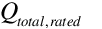 = total full-load heating
capacity of the coil at rated conditions (W)
= total full-load heating
capacity of the coil at rated conditions (W)
 = average defrost power
for the simulation time step (W)
= average defrost power
for the simulation time step (W)
 = capacity of the
resistive defrost heating element (W)
= capacity of the
resistive defrost heating element (W)
DefrostEIRTempModFac = energy input ratio modifier
curve applicable during defrost
Heating Operation[LINK]
For any simulation time step, the total heating capacity of
the DX unit is calculated as follows:
If the outdoor air dry-bulb temperature is below the
maximum temperature for defrost operation, then the total
heating capacity is further adjusted due to outdoor coil frost
formation based on the results of Equation and Equation or
.
In a similar fashion, the electrical power draw by the DX
unit (compressors plus outdoor coil fans) for any simulation
time step is calculated. For a reverse-cycle defrost strategy,
the additional heating load (Qdefrost)
generated during defrost operation is added to the heating
load being requested by adjusting the part-load ratio. If a
resistive defrost strategy is selected,
Qdefrost = 0. The part-load fraction
correlation for the heating coil (user input, Equation or ) is
used in the calculation of electrical power draw to account
for efficiency losses due to compressor cycling.
where
 = average compressor and
outdoor fan power for the simulation time step(W)
= average compressor and
outdoor fan power for the simulation time step(W)
 = total heating capacity
W, Eqn.
= total heating capacity
W, Eqn.
 = coefficient of
performance at rated conditions (user input)
= coefficient of
performance at rated conditions (user input)
InputPowerMultiplier = power adjustment due to
frost if applicable -Eqn. or
The crankcase heater is assumed to operate when the heating
coil’s compressor is OFF, and the average crankcase heater
power for the simulation time step is calculated as
follows:
where
= average crankcase
heater power for the simulation time step (W)
 = crankcase heater
capacity (W)
= crankcase heater
capacity (W)
If this heating coil is used as part of an air-to-air heat
pump (Ref. AirLoopHVAC:UnitaryHeatPump:AirToAir), the
crankcase heater defined for this DX heating coil is enabled
during the time that the compressor is not running for either
heating or cooling (and the crankcase heater power defined in
the DX cooling coil object is disregarded in this case). In
this instance, RTF in the above equations would be the runtime
fraction of the heat pump’s heating coil or cooling coil,
whichever is greater.
The properties of the air leaving the heating coil at
full-load operation are calculated using the following
equations:
where
 = enthalpy of the air
leaving the heating coil (J/kg)
= enthalpy of the air
leaving the heating coil (J/kg)
 = leaving air humidity
ratio (kg/kg)
= leaving air humidity
ratio (kg/kg)
 = leaving air dry-bulb
temperature (°C)
= leaving air dry-bulb
temperature (°C)
PsyTdbFnHW = EnergyPlus psychrometric function,
returns dry-bulb temp given enthalpy and humidity ratio
Condenser Inlet Air
Temperature[LINK]
The air temperature entering the outdoor condenser is based
on the weather data used during a simulation. This temperature
is either taken directly from the weather data, or can be
adjusted based on the height of the outdoor condenser. Since
this DX heating coil can only be used in conjunction with a DX
cooling coil, the input for Condenser Air Inlet Node Name in
the DX cooling coil object can be used to control this
optional feature. If this input is left blank, the air
temperature entering the condenser is based soley on the
weather data. If this input is not blank, then the node name
specified must also be listed in an OutdoorAir:Node
or OutdoorAir:NodeList
object. When the node name is listed in an OutdoorAir:NodeList
object, the air temperature entering the condenser is based
soley on the weather data. When the node name is listed in an
OutdoorAir:Node
object, the height of the node determines the air temperature
entering the outdoor condenser (see description of Local
Outdoor Air Temperature Calculation in the Atmospheric
Variation section of this document for further details).
Supply
Air Fan Control: Cycling vs. Continuous[LINK]
One of the inputs to the DX coil model is the supply air
fan operation mode: cycling fan, cycling compressor
(CyclingFanAndCompressor) or continuous fan, cycling
compressor (ContinuousFanWithCyclingCompressor). The first
operation mode is frequently referred to as “AUTO fan”, where
the compressor(s) and supply air fan operate in unison to meet
the zone heating load, and cycle off together when the heating
load has been met. The second operation mode is often referred
to as “fan ON”, where the compressor(s) cycle on and off to
meet the zone heating load but the supply air fan operates
continuously regardless of compressor operation.
Since this DX heating coil can only be used in conjunction
with a DX cooling coil (i.e. heat pumps), and these coils are
used in AC equipment that specifies a fan operation mode
schedule (e.g AirLoopHVAC:UnitaryHeatPump:AirToAir), the
selection made in the DX heating coil is currently ignored and
the fan operation mode schedule value determines the fan
operation mode for each time step throughout the simulation. A
fan operation mode schedule value of 0 specifies AUTO fan mode
operation while values other than 0 specify fan ON operation.
The use of a schedule allows the fan operation mode to change
based on time-of-day or with changes in season.
The EnergyPlus methodology for determining the impact that
HVAC equipment has on an air stream is to calculate the mass
flow rate and air properties (e.g., enthalpy, dry-bulb
temperature, humidity ratio) exiting the equipment. These
exiting conditions are passed along as inlet conditions to the
next component model in the air stream. Eventually the flow
rate and properties of the air being supplied to the
conditioned zone are used in the zone energy balance to
determine the resulting zone air temperature and humidity
ratio.
With this methodology, the determination of the air mass
flow rate and air properties for the two different supply air
fan operation modes is slightly different. For the case of
cycling fan/cycling compressor, the conditions of the air
leaving the heating coil are the steady-state values
calculated using equations , and above. However the air mass
flow rate passed along to the next component (and eventually
to the conditioned zone) is the average air mass flow rate for
the system simulation time step (determined by the heating
system; see AirLoopHVAC:UnitaryHeatPump:AirToAir). For this
fan control type, the heating coil part-load fraction
(Equation or ) is also passed to Fan:OnOff
(if used) to properly calculate the supply air fan power and
associated fan heat.
For the case of continuous fan/cycling compressor, the air
mass flow rate is constant. However, the air properties
leaving the heating coil are calculated as the average
conditions during the system simulation time step. The model
assumes that the exiting air conditions are the steady-state
values calculated using equations , and above when the
compressor(s) operate. For the remainder of the system
simulation time step, it is assumed that the air exiting the
DX coil has the same properties as the air entering the coil.
For this supply air fan operating strategy, the leaving air
properties are calculated as follows:
DOE. 1982. DOE-2 engineers manual, version 2.1A.
LBL-11353. Berkeley, CA: Lawrence Berkeley National
Laboratory.
ESTSC. 2001. DOE-2.1E Version
110 (source code). Oak Ridge, TN: Energy Science and
Technology Software Center.
Miller, R.L. and Jaster, H. 1985. Performance of Air-Source
Heat Pumps. EM-4226. Palo Alto, CA: Electric Power Research
Institute.
Single-Speed
DX Heating Coil Standard Ratings[LINK]
For single-speed direct expansion (DX) heating coils, the
industry standard ratings of High Temperature Heating Standard
(Net) Rating Capacity, Low Temperature Heating Standard (Net)
Rating Capacity and Heating Seasonal Performance Factor (HSPF)
are calculated according to ANSI/AHRI Standard 210/240 (AHRI
2008).
For the Coil:Heating:DX:SingleSpeed
object in EnergyPlus, these standard ratings are not direct
inputs to the model. However, these standard ratings can be
calculated using user-entered information for the Coil:Heating:DX:SingleSpeed
object. These standard rating values are provided in the
eplusout.eio output file (Ref. OutputDetailsAndExamples.pdf)
and also in the predefined tabular output reports
(Output:Table:SummaryReports object, Equipment Summary).
Currently, the standard ratings are only calculated and output
for single-speed DX heating coils. If the multi-speed DX
heating coil is specified, then no standard ratings are output
from EnergyPlus at this time.
Note: The standard ratings described in this section
require that the DX heating coil model be evaluated at
specific operating conditions (i.e., specific temperatures for
air entering the heating coil and for air entering the
air-cooled [outdoor] condenser). If the heating coil
performance curves can not be evaluated at the required test
conditions, then a standard rating value will be calculated at
user specified curve limit as an output and a warning message
will written to eplusout.err. For example, if the curve object
(Curve:Biquadratic) for Total Heating Capacity Function of
Temperature Curve has a minimum value of -5C for dry-bulb
temperature entering the condenser coil, the HSPF calculation
requires that heating capacity and EIR be calculated at
-8.33C, so this would result in HSPF value calculated at -5C
as an output and a warning message in the eplusout.err
file.
High
Temperature Heating Standard (Net) Rating Capacity[LINK]
The procedure for calculating the Standard Rating Heating
Capacity is given by:
where,
 = Total standard (net)
heating capacity (W) of the air-source heat pump equipment in
heating mode determined from ANSI/AHRI Standard 210/240 and
test conditions shown in Table 52. The standard heating test
conditions for air-cooled condenser are: indoor coil entering
air dry-bulb 21.1°C and outdoor coil entering air dry-bulb
8.33°C.
= Total standard (net)
heating capacity (W) of the air-source heat pump equipment in
heating mode determined from ANSI/AHRI Standard 210/240 and
test conditions shown in Table 52. The standard heating test
conditions for air-cooled condenser are: indoor coil entering
air dry-bulb 21.1°C and outdoor coil entering air dry-bulb
8.33°C.
 =Total standard heating
capacity (W) of the air-source heat pump equipment in heating
mode determined from ANSI/AHRI Standard 210/240 and test
conditions shown in Table 46. The standard heating test
conditions for air-cooled condenser are: indoor coil entering
air dry-bulb 21.1°C and outdoor coil entering air dry-bulb
8.33°C.
=Total standard heating
capacity (W) of the air-source heat pump equipment in heating
mode determined from ANSI/AHRI Standard 210/240 and test
conditions shown in Table 46. The standard heating test
conditions for air-cooled condenser are: indoor coil entering
air dry-bulb 21.1°C and outdoor coil entering air dry-bulb
8.33°C.
 = Rated total heating
capacity, user input (W)
= Rated total heating
capacity, user input (W)
 = User-specified
bi-quadratic curve evaluated at the indoor coil entering air
dry-bulb 21.1°C and outdoor coil entering air dry-bulb 8.33°C
for air-cooled condenser as specified in Table 52,
(dimensionless).
= User-specified
bi-quadratic curve evaluated at the indoor coil entering air
dry-bulb 21.1°C and outdoor coil entering air dry-bulb 8.33°C
for air-cooled condenser as specified in Table 52,
(dimensionless).
= Supply air fan power at
rated conditions, (W). The Rated Indoor Coil Fan Power Per
Volume Flow rate is a user-entered value, with a default of
775 W/(m3/s)) if the user leaves this input field blank. The
default value is taken from ANSI/ASHRAE Standard 210/240-2008
where it is defined for systems which do not have an Indoor
Coil fan furnished as part of the system. See the description
given at the end of this section for how this value is
calculated.
Low
Temperature Heating Standard (Net) Rating Capacity[LINK]
The procedure for calculating the Low Temperature Standard
Rating Heating Capacity is given by:
where,
 =Total standard (net)
heating capacity (W) of the air-source heat pump equipment in
heating mode determined from ANSI/AHRI Standard 210/240 and
test conditions shown in Table 46. The standard heating test
conditions for air-cooled condenser are: indoor coil entering
air dry-bulb 21.1°C and outdoor coil entering air dry-bulb
(-8.33) °C.
=Total standard (net)
heating capacity (W) of the air-source heat pump equipment in
heating mode determined from ANSI/AHRI Standard 210/240 and
test conditions shown in Table 46. The standard heating test
conditions for air-cooled condenser are: indoor coil entering
air dry-bulb 21.1°C and outdoor coil entering air dry-bulb
(-8.33) °C.
 =Total standard heating
capacity (W) of the air-source heat pump equipment in heating
mode determined from ANSI/AHRI Standard 210/240 and test
conditions shown in Table 52. The standard heating test
conditions for air-cooled condenser are: indoor coil entering
air dry-bulb 21.1°C and outdoor coil entering air dry-bulb
(-8.33) °C.
=Total standard heating
capacity (W) of the air-source heat pump equipment in heating
mode determined from ANSI/AHRI Standard 210/240 and test
conditions shown in Table 52. The standard heating test
conditions for air-cooled condenser are: indoor coil entering
air dry-bulb 21.1°C and outdoor coil entering air dry-bulb
(-8.33) °C.
= Rated total heating
capacity, user input (W)
 = User-specified
bi-quadratic curve evaluated at the indoor coil entering air
dry-bulb 21.1°C and outdoor coil entering air dry-bulb (-8.33)
°C for air-cooled condenser as specified in Table 46,
(dimensionless).
= User-specified
bi-quadratic curve evaluated at the indoor coil entering air
dry-bulb 21.1°C and outdoor coil entering air dry-bulb (-8.33)
°C for air-cooled condenser as specified in Table 46,
(dimensionless).
= Supply air fan power at
rated conditions, (W). The Rated Indoor Coil Fan Power Per
Volume Flow rate is a user-entered value, with a default of
775 W/(m3/s)) if the user leaves this input field blank. The
default value is taken from ANSI/ASHRAE Standard 210/240-2008
where it is defined for systems which do not have an Indoor
Coil fan furnished as part of the system. See the description
given at the end of this section for how this value is
calculated.
Heating Seasonal Performance Factor (HSPF) is defined as
the total space heating required during the space heating
season, divided by the total electrical energy consumed by the
heat pump system during the same season.
Calculations of HSPF of a heat pump having a single-speed
compressor that was tested with a fixed speed indoor fan
installed, a constant-air-volume-rate indoor fan installed, or
with no indoor fan installed is given below.
Where,
 = The ratio of the
electrical energy consumed by the heat pump during periods of
the space heating season when the outdoor temperature fell
within the range represented by bin temperature
= The ratio of the
electrical energy consumed by the heat pump during periods of
the space heating season when the outdoor temperature fell
within the range represented by bin temperature  to the total number of hours in
the heating season (N), W.
to the total number of hours in
the heating season (N), W.
 = The ratio of the
electrical energy used for resistive space heating during
periods when the outdoor temperature fell within the range
represented by bin temperature to the total number of hours in
the heating season (N),W.
= The ratio of the
electrical energy used for resistive space heating during
periods when the outdoor temperature fell within the range
represented by bin temperature to the total number of hours in
the heating season (N),W.
= The outdoor bin
temperature, °C. Outdoor temperatures are “binned” such that
calculations are only performed based one temperature within
the bin. Bins of 2.78 °C are used.
 = Fractional bin hours
for the heating season; the ratio of the number of hours
during the heating season when the outdoor temperature fell
within the range represented by bin temperature to the total number of hours in
the heating season, dimensionless. Obtain values from Table 17 of AHRI Std.
210/240-2008 (Table 53 below).
= Fractional bin hours
for the heating season; the ratio of the number of hours
during the heating season when the outdoor temperature fell
within the range represented by bin temperature to the total number of hours in
the heating season, dimensionless. Obtain values from Table 17 of AHRI Std.
210/240-2008 (Table 53 below).
 = The bin number,
dimensionless.
= The bin number,
dimensionless.
 = For each generalized
climatic region, the total number of temperature bins,
dimensionless. Referring to Table 17, is the highest bin number ( ) having a nonzero entry for the
fractional bin hours for the generalized climatic region of
interest.
= For each generalized
climatic region, the total number of temperature bins,
dimensionless. Referring to Table 17, is the highest bin number ( ) having a nonzero entry for the
fractional bin hours for the generalized climatic region of
interest.
 = The demand defrost
credit described in section 3.9.2 of AHRI Std. 210/240-2008,
dimensionless. For simplification, assigned a value of 1 for
timed defrost control and a value of 1.03 for demand defrost
control.
= The demand defrost
credit described in section 3.9.2 of AHRI Std. 210/240-2008,
dimensionless. For simplification, assigned a value of 1 for
timed defrost control and a value of 1.03 for demand defrost
control.
 = The building space
conditioning load corresponding to an outdoor temperature
of ; the heating season
building load also depends on the generalized climatic
region’s outdoor design temperature and the design heating
requirement, W.
= The building space
conditioning load corresponding to an outdoor temperature
of ; the heating season
building load also depends on the generalized climatic
region’s outdoor design temperature and the design heating
requirement, W.
Building
heating load can be evaluated by using the following
equation
Where,
 = The outdoor design
temperature, °C. An outdoor design temperature is specified
for each generalized climatic region in Table 17 of AHRI Std.
210/240-2008 (Table 53 below).
= The outdoor design
temperature, °C. An outdoor design temperature is specified
for each generalized climatic region in Table 17 of AHRI Std.
210/240-2008 (Table 53 below).
 = 0.77, a correction
factor which tends to improve the agreement between calculated
and measured building loads, dimensionless.
= 0.77, a correction
factor which tends to improve the agreement between calculated
and measured building loads, dimensionless.
 = Design Heating
Requirement, W. This is the amount of heating required to
maintain a given indoor temperature at a particular outdoor
design temperature.
= Design Heating
Requirement, W. This is the amount of heating required to
maintain a given indoor temperature at a particular outdoor
design temperature.
For a single speed heat pump with a fixed speed indoor fan
installed, a constant-air-volume-rate indoor fan installed, or
with no indoor fan installed, the minimum and maximum design
heating requirements for each generalized climatic region can
be calculated as follows:
Both  and
and  above should be rounded to the
nearest standardized DHR given in Table 54.
above should be rounded to the
nearest standardized DHR given in Table 54.
The intermediate term used in the calculations of HSPF can
be calculated using the equations described below.
Where,
whichever is less; the heating mode load factor for
temperature bin  ,
dimensionless.
,
dimensionless.
 = the space heating
capacity of the heat pump when operating at outdoor
temperature
= the space heating
capacity of the heat pump when operating at outdoor
temperature  , W.
, W.
 = the electrical power
consumption of the heat pump when operating at outdoor
temperature
= the electrical power
consumption of the heat pump when operating at outdoor
temperature  , W.
, W.
 = the heat pump low
temperature cut-out factor, dimensionless.
= the heat pump low
temperature cut-out factor, dimensionless.
 = the part load factor,
dimensionless.
= the part load factor,
dimensionless.
Part load factor is determined as follows:
Where,
 = Degradation coefficient
which is defaulted to the value of 0.25
= Degradation coefficient
which is defaulted to the value of 0.25
Low temperature cut-out factor is determined as follows:
where,
 = the outdoor temperature
when the compressor is automatically shut off, °C. (If no such
temperature exists,
= the outdoor temperature
when the compressor is automatically shut off, °C. (If no such
temperature exists,  is
always greater than and
is
always greater than and ).
).
= the outdoor temperature
when the compressor is automatically turned back on, if
applicable, following an automatic shut-off, °C.
Calculate 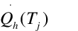 and
and  using,
 and
and  are the (net)
values calculated using performance curves entered by the user
and supply fan power per rated air flow rate.
are the (net)
values calculated using performance curves entered by the user
and supply fan power per rated air flow rate.
Heating Mode Test Conditions for Units Having a
Single-Speed Compressor and a Fixed-Speed Indoor Fan, a
Constant Air Volume Rate Indoor Fan, or No Indoor
Fan
| <> |
| Test description |
| H1 Test (Required, Steady) |
| H1C Test (Required, Steady) |
| H2 Test (Required, Steady) |
| H3 Test (Required, Steady) |
| Notes: |
Generalized Climatic Region Information
| <> |
| Region Number |
| Heating Load Hours, HLH |
Outdoor Design Temperature,  (°C) (°C) |
 |
| 1 |
| 2 |
| 3 |
| 4 |
| 5 |
| 6 |
| 7 |
| 8 |
| 9 |
| 10 |
| 11 |
| 12 |
| 13 |
| 14 |
| 15 |
| 16 |
| 17 |
| 18 |
| * Pacific Coast Region |
Standardized Design Heating Requirements
(W)
| <> |
| 1465.356 |
| 2930.712 |
| 4396.068 |
| 5861.424 |
Multi-Speed
Electric Heat Pump DX Air Heating Coil[LINK]
This model (object name Coil:Heating:DX:MultiSpeed:)
simulates the performance of an air-to-air direct expansion
(DX) heating system. The main difference compared to the other
heating coil model (Coil:Heating:DX:SingleSpeed) is that this
heating coil allows modeling of two to four discrete
compressor speeds. Each speed has a set of corresponding
performance information at rated conditions along with curve
fits for variations in total capacity, energy input ratio and
part-load fraction to determine the performance of the unit at
part-load conditions (DOE 1982). The full load supply airflow
rate is dependent on the speed number and is set by its parent
object (Ref: AirLoopHVAC:UnitaryHeatPump:AirToAir:MultiSpeed).
The part-load impact on coil energy use is automatically
applied to the lowest speed. A choice is provided to determine
whether part-load impacts on coil energy use are applied when
the coil is operating at speeds greater than Speed 1.
Adjustment factors applied to total capacity and input power
to account for frost formation on the outdoor coil are
calculated at each speed.
This model simulates the thermal performance of the indoor
DX heating coil, and the power consumption of the outdoor unit
(multispeed compressor, fans, crankcase heaters and defrost
heaters). The performance of the indoor supply air fan varies
widely from system to system depending on control strategy
(e.g., constant fan vs. AUTO fan), fan type, fan motor
efficiency and pressure losses through the air distribution
system. Therefore, this DX system model does not account for
the thermal effects or electric power consumption of the
indoor supply air fan. EnergyPlus contains separate models for
simulating the performance of various indoor fan
configurations, and these models can be easily linked with the
DX system model described here to simulate the entire DX
system being considered. For the time being, this coil model
can only be called by the parent object AirLoopHVAC:UnitaryHeatPump:AirToAir:MultiSpeed.
When the model determines performance at Speed 1 (the
lowest speed) or cycling between OFF and Speed 1, its
performance is almost the same as the performance for the Coil:Heating:DX:SingleSpeed
model. However, the outlet conditions are calculated slightly
differently. Therefore, the Coil:Heating:DX:SingleSpeed
model may be considered as a subset of the model described
here. When the multispeed coil model determines performance at
higher speeds (above 1), the model linearly interpolates the
performance at two consecutive speeds (n-1 and n) as needed to
meet the heating load, with the fraction of time at each speed
established by the speed ratio.
The model inputs are also very similar to the inputs of the
Coil:Heating:DX:SingleSpeed
object. The main difference is that this multispeed model
requires a set of fields at each speed, such as rated
capacity, rated COP, two capacity modifiers, two energy input
ratio modifiers, and part-load correction. The inputs also
include waste heat fraction and modifier as a function of
temperature to calculate recoverable waste heat for heat
recovery, which are not available in the similar Coil:Heating:DX:SingleSpeed
object.
Speed 1 Operation[LINK]
The calculation procedures in this model, including defrost
and crankcase heater, are indentical to the Coil:Heating:DX:SingleSpeed
object (Ref: Coil:Heating:DX:SingleSpeed) with one exception:
outlet node condition calculation when the supply air fan
operation mode is ContinuousFanWithCyclingCompressor. The
following procedure provides the detailed description of the
exception.
- Total delivered heating capacity
The total delivered heating capacity for speed 1 operating
at the cycling ratio needed to meet the requested heating load
is:
where,
Qcoil,cycling= delivered sensible
heating capacity for Speed 1 operating at a specific cycling
ratio [W]
= air mass flow rate
through heating coil at Speed 1 as set by the parent object
[kg/s]
houtlet,full= specific enthalpy of the
coil outlet air during full-load operation at Speed 1 (no
cycling) [J/kg]
hinlet= specific enthalpy of the coil inlet
air [J/kg]
CycRatio= cycling ratio at Speed 1, ratio of
requested heating load to the full-load capacity of the coil
at Speed 1 [dimensionless]
It is assumed that the coil provides no heating capacity
when the coil is OFF, even if the supply air fan continues to
operate.
- Outlet air specific enthalpy
The average specific enthalpy of the coil outlet air is
then calculated based on the delivered sensible heating
capacity and the average air mass flow rate entering the
coil:
where,
houtlet,average= average specific
enthalpy at the coil outlet [J/kg]
= mass flow rate at the
inlet to the coil as established by the parent object (Ref. AirLoopHVAC:UnitaryHeatPump:AirToAir:MultiSpeed,
Mass Flow Rate Calculation). This flow rate is the average
value determined by the parent object, accounting for the
specified flow rate when the heating coil is ON and the
specified flow rate when the heating coil is OFF for the time
step being simulated.
The heating coil’s outlet air humidity ratio equals the
inlet air humidity ratio since the coil does not change the
moisture content of the air. So the average outlet air
temperature is calculated based on the inlet air humidity
ratio and the average outlet air enthalpy using the
psychrometric function PsyTdbFnHW.
The main reason for using the above approach is that outlet
air conditions are calculated in the same way for all
operating speeds.
The crankcase heater defined for this DX heating coil is
enabled during the time that the compressor is not running for
either heating or cooling. The crankcase heater power use from
either heating or cooling is reported in the heating coil.
Higher Speed Operation[LINK]
This section describes how higher speed operation is
simulated. When the required sensible load is less than the
full load sensible capacity at Speed n (Speed Number > 1),
the following calculations are performed:
- Total delivered heating capacity at Speed n-1 and Speed
n


where,
TotCapi= total delivered heating
capacity at given temperatures and flow rates at Speed i
[W]
RatedCapi= heating capacity at the
rated conditions at Speed i [W]
TotCapTempModFaci~~= total heating
capacity modifier as a function of indoor and outdoor air
dry-bulb temperature at Speed i
TotCapFlowModFaci~~= total heating
capacity modifier as a function of the ratio of the actual
flow rate across the heating coil to the rated airflow rate at
Speed i
i= Speed n or Speed n-1
- EIR at Speed n-1 and Speed n
where,
EIRi= energy input ratio at given
temperatures and flow rates at Speed i [W]
RatedEIRi= energy input ratio at the
rated conditions at Speed i [W]
EIRTempModFaci~~= energy input ratio
modifier as a function of indoor and outdoor air dry-bulb
temperature at Speed i
EIRFlowModFaci~~= energy input ratio
modifier as a function of the ratio of the actual flow rate
across the heating coil to the rated airflow rate at Speed
i
i= Speed n or Speed n-1
- Full load outlet air specific enthalpy at Speed n-1 and
Speed n
where,
HeatingCapacityMultiplier= frost adjustment factor
for heating capacity (See Ref.
Coil:Heating:DX:SingleSpeed)
houtlet,full_Speedn= specific enthalpy
of the coil outlet air during full-load operation at Speed n
(no cycling) [J/kg]
houtlet,full_Speedn-1= specific
enthalpy of the coil outlet air during full-load operation at
Speed n-1 (no cycling) [J/kg]
- Effective total heating capacity
where,
= delivered sensible
heating capacity at a given speed ratio between two
consecutive speeds [W]
= air mass flow rate
through heating coil at Speed n as set by the parent object
[kg/s]
= air mass flow rate
through heating coil at Speed 1 as set by the parent object
[kg/s]
- Average outlet air enthalpy
where,
houtlet,average= average specific
enthalpy at the coil outlet [J/kg]
hinlet= specific enthalpy of the coil inlet
air [J/kg]
= Mass flow rate at the
inlet to the coil as established by the parent object (Ref. AirLoopHVAC:UnitaryHeatPump:AirToAir:MultiSpeed,
Mass Flow Rate Calculation). This flow rate is the average
value determined by the parent object, accounting for the
specified flow rate when the heating coil is at Speed n and
the specified flow rate when the heating coil is at Speed n-1
for the time step being simulated.
- Average outlet air temperature
The heating coil’s outlet air humidity ratio equals the
inlet air humidity ratio since the coil does not change the
moisture content of the air. So the average outlet air
temperature is calculated based on the inlet air humidity
ratio and the average outlet air enthalpy using the
psychrometric function PsyTdbFnHW.
- Full load energy inputs at Speed n-1 and Speed n
where,
InputPowerMultiplier= Frost adjustment factor for
heating power calculation (Ref.
Coil:Heating:DX:SingleSpeed)
- Calculate combined energy input
When the input for the field ‘Apply Part Load Fraction to
Speeds Greater than 1’ is No (equivalent to a single
compressor), the combined energy output is calculated as
follows:
When the input for the field ‘Apply Part Load Fraction to
Speeds Greater than 1’ is Yes (equivalent to multiple
compressors), the combined energy output is calculated as
follows:
where,
HeatingPower= Power used in Watt
RTF= Run time fraction (SpeedRatio/Part-load Fraction) at
Speed n
When the defrost strategy is resistive, the power
calculation is the same as Speed 1 operation (Ref.
Coil:Heating:DX:SingleSpeed). When the defrost strategy is
reverse-cycle, the following calculations are performed:
where:
 = additional indoor
heating load due to reverse-cycle defrost at Speed n
(W)
= additional indoor
heating load due to reverse-cycle defrost at Speed n
(W)
 = total full-load heating
capacity of the coil at rated conditions at Speed n (W)
= total full-load heating
capacity of the coil at rated conditions at Speed n (W)
 = full load defrost power
for the simulation time step at Speed n-1 (W)
= full load defrost power
for the simulation time step at Speed n-1 (W)
 = full load defrost power
for the simulation time step at Speed n (W)
= full load defrost power
for the simulation time step at Speed n (W)
 = capacity of the
resistive defrost heating element at Speed n-1 (W)
= capacity of the
resistive defrost heating element at Speed n-1 (W)
 = capacity of the
resistive defrost heating element at Speed n (W)
= capacity of the
resistive defrost heating element at Speed n (W)
DefrostEIRTempModFac= defrost energy input ratio (EIR)
modifier curve (Ref. Coil:Heating:DX:SingleSpeed).
Tfrac,defrost= fractional defrost time (Ref.
Coil:Heating:DX:SingleSpeed)
When the input for the field ‘Apply Part Load Fraction to
Speeds Greater than 1’ is No (equivalent to a single
compressor), the average defrost power is calculated as
follows:
When the input for the field ‘Apply Part Load Fraction to
Speeds Greater than 1’ is Yes (equivalent to multiple
compressors), the combined defrost energy is calculated as
follows:
where,
 = average defrost power
used in Watt
= average defrost power
used in Watt
RTF= Run time fraction (SpeedRatio/Part-load Fraction) at
Speed n
There is no power need at higher speed operation.
Waste heat calculation[LINK]
The waste heat generated by this coil object is calculated
as:
where
Fraction= rated waste heat fraction of the energy input
TempModifier= waste heat modifier as a function of indoor
and outdoor air dry-bulb temperature
See the references for the single speed DX heating coil
earlier in this document.
Variable Speed DX
Heating Coil[LINK]
The latest technology for commercial air conditioners and
air-to-air heat pumps can utilize a variable speed compressor
with a variable speed indoor blower and outdoor fan. The
indoor and outdoor air flow rates are usually a function of
the compressor speed. Refrigerant mass flow rate is a function
of compressor speed as well as outdoor heat exchanger entering
air temperature and indoor dry bulb or wet bulb. The control
system adjusts the equipment capacity based on zone
temperature measurements relative to the thermostat set point.
The control logic determines what compressor speed is required
to control to the zone temperature requirement in response to
increased or decreased capacity (heating or cooling load). The
compressor, fan and blower speeds are not discrete values and
can be considered to vary infinitesimally between the minimum
and maximum compressor speed. At the minimum compressor speed
(which is different for heating and cooling), for a continuous
fan, the supply airflow is fixed and the unit will have to
cycle for reduced part loads below this point. For a cycling
fan, the fan will cycle with the compressor.
Similar to variable-speed water source heat pump, we expand
the number of speed levels and the corresponding curve sets up
to ten. The number of speed levels is selectable by the user.
The user can provide speed levels at any number from 1 to 10.
In the case that the given speed levels are above 1, the model
would do linear interpolation between neighboring speeds. The
more curves, the more accurate. Furthermore, using linear
interpolation and inputting air flow rates at individual speed
levels facilitates arbitrary relationships of flow rate as a
function of the compressor speed level.
The Coil:Heating:DX:VariableSpeed
object will simulate the performance of a DX heating coil used
in combination with a variable-speed air-to-air heat pump. It
will fit into the parent objects of AirLoopHVAC:UnitaryHeatPump:AirToAir
and
ZoneHVAC:PackagedTerminalHeatPump,
etc.
The rated conditions for obtaining the capacities and COPs
are at indoor dry-bulb temperature of 21.1 ˚C (70 ˚F) and the
source side entering air temperature of 8.3 ˚C (47 ˚F). Some
equations are provided below to help explain the function of
the various performance curves and data fields.
Model Description[LINK]
The Coil:Heating:DX:VariableSpeed
object is modeled similar to Coil:Heating:WaterToAirHeatPump:VariableSpeedEquationFit.
Of course, rather than referencing a water source evaporator,
the new coil object references an air source and has
defrosting operation. The evaporator entering air temperature
is used in lieu of the entering water temperature.
It shall be noted for the capacity and flow rate inputs,
two fields are autosizable, which are Rated Heating Capacity
at the Selected Nominal Speed Level and the Rated Volumetric
Air Flow Rate at the Selected Nominal Speed Level. They are
used to scale the performances of a specific unit and
correlate with the actual loop flow. Except these two fields,
all other capacity and flow rate inputs at individual speed
levels should be directly obtained from Reference Unit catalog
data, specific to an actual unit.
The Rated Heating Capacity at Selected Nominal Speed Level
contains the rated capacity to match the building heating load
at the design day. The rated heating capacity is used to
determine a capacity scaling factor, as compared to the
Reference Unit capacity at the nominal speed level.
And then, this scaling factor is used to determine
capacities at rated conditions for other speed levels, as
below:
The Rated Volumetric Air Flow Rate is used to determine an
internal scaling factor, and calculate the air flow rates in
the parent objects, as follows:
And the loop volumetric air flow rates at various speed
levels in the parent objects are calculated as below:
If the volumetric air flow rate at one speed level is
higher than the flow rate allowed by the fan in the parent
object, the flow rate will be set back to the fan flow
rate.
If  equals unity, the loop
air flow rate becomes the design flow rate of the Reference
Unit (after scaled by the rated heating capacity). The Rated
Volumetric Air Flow Rate is introduced here to correlate with
the actual flow rate in the air loop, in case that it differs
from the design specification. Certainly, it is recommended
that the Rated Volumetric Air Flow Rate is selected in the way
that
equals unity, the loop
air flow rate becomes the design flow rate of the Reference
Unit (after scaled by the rated heating capacity). The Rated
Volumetric Air Flow Rate is introduced here to correlate with
the actual flow rate in the air loop, in case that it differs
from the design specification. Certainly, it is recommended
that the Rated Volumetric Air Flow Rate is selected in the way
that  is unity, so as to get
more accurate results from the performance curves.
is unity, so as to get
more accurate results from the performance curves.
This object includes 4 curve objects at each individual
speed level.
Total heating capacity modifier curve (function of
temperature).
Total heating capacity modifier curve (function of air
flow fraction).
Energy input ratio (EIR) modifier curve (function of
temperature).
Energy input ratio (EIR) modifier curve (function of
air flow fraction).
The flow fraction modifier curves are used as a
placeholder, to account for off-design flow rates if needed.
If the manufacturer doesn’t provide off-design performances,
we can simply use a default modification multiplier of
1.0.
At the lowest speed, there will be one additional
performance curve to account for the part-load condition,
i.e.
Part load fraction correlation (function of part load
ratio).
Total heating capacity modifier curve (function of
temperature)
The total heating capacity modifier as a function of
temperature curve (CAP-FT) is a biquadratic curve with two
independent variables: dry-bulb temperature of the air
entering the heating coil and the air DB temperature entering
the evaporator coil. The output of this curve is multiplied by
the rated total heating capacity at the speed, to give the
total heating capacity at the specific entering air
temperatures at which the ASHP unit is operating (i.e., at
temperatures different from the rating point
temperatures).
where
DBi = dry-bulb temperature of the air entering
the heating coil, °C
DBo = dry-bulb temperature of the air entering
the outdoor coil, °C
a-f = regression curve-fit coefficients
- Total heating capacity modifier curve (function of air
flow fraction)
where
ffa = actual air mass flow rate/design air mass
flow rate, at one speed level;
a-d = regression curve-fit coefficients, if no data
available for the correction, the user can simply put a = 1.0,
and the other coefficients as 0.0.
- Energy input ratio (EIR) modifier curve (function of
temperature)
The energy input ratio modifier curve as a function of
temperature (EIR-FT) is a biquadratic curve with two
independent variables DBi and DBo. The
output of this curve is multiplied by the rated EIR at the
speed (inverse of the rated COP), to give the EIR at the
specific entering air temperatures at which the ASHP coil unit
is operating (i.e., at temperatures different from the rating
point temperatures).
where
a-f = regression curve fit coefficients.
- Energy input ratio (EIR) modifier curve (function of air
flow fraction)
where
a-d = regression curve-fit coefficients, if no data
available for correction, the user can simply put a = 1.0, and
the other coefficients as 0.0.
- Part load fraction correlation (function of part load
ratio)
This field defines the name of a quadratic or cubic
performance curve (Ref: Performance Curves) that parameterizes
the variation of electrical power input to the unit as a
function of the part load ratio (PLR, heating
load/steady-state heating capacity for Speed 1),
And
RTF = (PLR/PartLoadFrac) = runtime fraction of the heating
coil.
The part load fraction (PLF) correlation accounts for
efficiency losses due to compressor cycling. The part load
fraction correlation should be normalized to a value of 1.0
when the part load ratio equals 1.0 (i.e., no efficiency
losses when the compressor runs continuously for the
simulation timestep). For PLR values between 0 and 1 (0 <=
PLR < 1), the following rules apply:
PLF >= 0.7 and PLF >= PLR
If PLF < 0.7, the program resets the PLF value to 0.7,
and the simulation proceeds. The runtime fraction of the coil
is defined as PLR/PLF. If PLF < PLR, the runtime fraction
of the coil is limited to 1.0. A typical part load fraction
correlation would be:
If the user wishes to model no efficiency degradation due
to compressor cycling, the part load fraction correlation
should be defined as follows:
Lowest Speed Operation:[LINK]
The lowest speed operation of the variable-speed DX heating
coil is similar to the single speed DX heating coil. The total
(gross) heating capacity of the variable-speed DX coil is
calculated as follows:
And the EIR is calculated as:
And the power consumption including the compressor, outdoor
fan and accessories (not including indoor fan power) is,
The fraction of the actual air mass flow to the design air
mass flow rate is calculated:
Higher Speed Operation:[LINK]
At the speed level between the lowest and the highest,
there is no part-load loss. A parameter of speed ratio
(SpeedRatio) is used to define the capacity partition between
Speed x-1 and Speed x.
The design air flow rate at the speed ratio are given as
following:
And the fractions of air flow is given:
 =
=  = actual air mass flow
rate/DesignAirFlowRateSpeedRatio
= actual air mass flow
rate/DesignAirFlowRateSpeedRatio
The total heating capacities and EIRs at Speed x-1 and
Speed x are given:
The total heating capacity at the corresponding speed ratio
is:
And the power consumption is
The total amount of heat absorbed by the outdoor evaporator
is calculated as:
At last,
If the speed reaches the highest level, the speed ratio
becomes 1.0, and Speed x represents the highest speed.
Defrost Operation:[LINK]
The defrost operation of a variable-speed DX heating coil
is treated the same as the single-speed DX heating coil,
except using the total heating capacity at the max speed level
to replace the rated heating capacity of the single-speed DX
coil, when a reverse-cycle defrost strategy is specified.
We keep the defrost energy input ratio (EIR) modifier curve
(function of temperature) as the single speed DX heating coil.
It is a biquadratic curve with two independent variables:
outdoor air dry-bulb temperature and the heating coil entering
air wet-bulb temperature. The output of this curve is
multiplied by the heating coil capacity, the fractional
defrost time period and the runtime fraction of the heating
coil to give the defrost power at the specific temperatures at
which the coil is operating. This curve is only required when
a reverse-cycle defrost strategy is specified.
where
WBi = wet-bulb temperature of the air entering
the indoor coil, °C
DBo = dry-bulb temperature of the air entering
the outdoor coil, °C
a-f = regression curve-fit coefficients
Crankcase Heater
Operation:[LINK]
It is the same as the single-speed DX heating coil.
Desuperheater-Recovery-Based
Air Heating Coil[LINK]
The input object Coil:Heating:Desuperheater
provides a model that simulates the thermal performance of a
refrigerant-to-air heating coil and the parasitic electric
consumption of its control valves or other auxiliary devices.
The model assumes that the heating energy provided by this
coil is reclaimed from the superheated refrigerant gas leaving
a compressor and does not impact the performance of the
compressor. The objects from which this coil can obtain its
heating energy are:
Coil:Cooling:DX:SingleSpeed
Coil:Cooling:DX:TwoSpeed
Coil:Cooling:DX:TwoStageWithHumidityControlMode
Refrigeration:CompressorRack
Refrigeration:Condenser* (multiple objects)
The heat reclaim recovery efficiency (specified by the
user) defines the amount of heat available for use by this
coil. Approximately 25-30% of the energy rejected by typical
refrigeration system condensers is to reduce the superheated
refrigerant vapor temperature to the condensing temperature.
Recovery efficiencies higher than 30% may cause the
refrigerant gas to condense which in turn impacts the
performance of the refrigeration compressor rack. For this
reason, the maximum heat reclaim recovery efficiency for this
coil for all sources except the Refrigeration:Condenser:(Air,
Water, or Evap)Cooled is 30%.For these refrigeration
condensers, the amount of waste energy available in the
superheat region is explicitly calculated, so for these
condensers the maximum heat recovery efficiency is 90% of this
superheat energy. Also, for these refrigeration condensers, an
estimate of the temperature of the reclaimed heat source is
made and compared to the inlet air temperature for the coil.
If the reclaimed heat source is too cool, the amount of
available reclaim energy is set to zero.
NOTE: When the heating source is a refrigeration compressor
rack, the heat rejection location in the Refrigeration:CompressorRack
object must be “Outdoors”. If the compressor rack heat
rejection location is “Zone”, the total amount of heat
rejection available for reclaim (e.g., by this desuperheater
heating coil) is set to zero by the compressor rack object and
the simulation proceeds.
The sources for the waste heat can also be used to supply
other coils. To avoid double-counting this waste heat, the
amount available is corrected to reflect these other uses. For
the three DX Cooling Coil sources, this correction is made
within the same time step loop. For the two refrigeration
system sources, the correction is made using the value from
the previous time step.
The desuperheater heating coil can be used in air loop
simulations for various air heating applications. For example,
it can be used as an air reheat coil for high humidity control
in the compound objects AirLoopHVAC:Unitary:Furnace:HeatCool
and AirLoopHVAC:UnitaryHeatCool
(see High Humidity Control With HeatCool Configuration). For
this application, the desuperheater coil is controlled based
on the calculated heating load to maintain the zone
temperature and humidity setpoints (load-based control). The
source of reclaimed heat could be the direct expansion (DX)
cooling coil itself (Coil:Cooling:DX:SingleSpeed) or a
refrigerated case compressor rack
(Refrigeration:CompressorRack).
The desuperheater heating coil can also be used with
cooling/heating systems that maintain specific air loop (deck)
temperatures. For example, Figure 159 shows a schematic
diagram of the desuperheater heating coil used in conjunction
with the AirLoopHVAC:UnitaryCoolOnly object. The desuperheater
heating coil must be placed downstream of the DX cooling coil
when reclaiming heat from that cooling coil’s compressor(s).
Desuperheating heating coil placement is unrestricted when
reclaiming heat from a refrigeration compressor rack or
refrigeration condenser. The configuration in Figure 159 shows
the heating coil being controlled via a temperature-based
strategy. In this example, the DX cooling coil could be used
to the maintain its discharge air temperature at 11°C for zone
dehumidification. The desuperheater heating coil could then
raise the air dry-bulb temperature to 16°C providing a dry
supply air stream at a temperature which does not require much
additional heating by terminal units to meet the zone
temperature setpoint.
Since the heating provided by the desuperheater coil is
based on available waste heat from another system, the
selection of fan control for the air loop equipment is
essential for proper modeling. When the coil’s heating source
is a direct expansion cooling coil
(Coil:Cooling:DX:SingleSpeed, Coil:Cooling:DX:TwoSpeed,
or Coil:Cooling:DX:TwoStageWithHumidityControlMode), the air
loop’s fan control mode may be auto fan (cycling fan cycling
coil), constant fan, or variable volume since the
desuperheater heating coil cycles on/off with the DX cooling
coil. When the heating source is a compressor rack or
condenser for refrigerated cases, the supply air fan control
should be either variable volume or constant fan since the
desuperheater heating coil will typically be available the
entire simulation time step.
NOTE: Use of the desuperheater heating coil in variable air
volume systems should be done with caution since the model
assumption of a fixed heat reclaim recovery efficiency may not
be valid if the air flow rate over the coil varies
significantly.
The following sections describe the calculations used for
both the load-based and temperature-based strategies that can
control the desuperheater heating coil.
A minimum of seven inputs must be defined for the
desuperheater heating coil. The user must input the coil’s
name, an availability schedule name, and the heat reclaim
recovery efficiency (default of 25%, with a range of 0% to 30%
except for detailed refrigeration condensers which have a
default of 80%, with a range of 0% to 90%). The next two
inputs are the heating coil’s inlet and outlet air node names.
The user must also enter the desuperheater heat source type
and name which are validated when the model inputs are read
into the program.
The final two fields are optional. The first of these is
the coil temperature setpoint node name. This field is used
when the desuperheater heating coil is controlled based on an
air loop temperature and a setpoint manager (Ref.
SetpointManager:*) is used to place a temperature setpoint on
this air node. The latter of these optional fields is the
parasitic electric load. This field allows the user to define
the electric energy use of parasitic equipment associated with
the desuperheater heating coil (e.g. control valves).
Model Description[LINK]
The model calculates the thermal performance of the heating
coil based on the control strategy used. When a temperature
setpoint node name is not entered, the control type is assumed
to be load-based operation. This method should be used when
this coil is specified as the air reheat coil for high
humidity control with the compound object AirLoopHVAC:Unitary:Furnace:HeatCool
or AirLoopHVAC:UnitaryHeatCool.
If the temperature setpoint node name is entered, the control
type is temperature-based operation. This method is used when
the heating coil is controlled to maintain a dry-bulb
temperature setpoint in an air loop.
Load-Based Operation[LINK]
When load-based operation is selected, a load to be met by
the heating coil is requested by the parent object (e.g.,
AirLoopHVAC:Unitary:Furnace:HeatCool). The model first
calculates the heating coil capacity based on the total
condenser waste heat rejected by the heating source.
where:
 = heating capacity of the
desuperheater coil (W)
= heating capacity of the
desuperheater coil (W)
 = total amount of
condenser waste heat rejected by the heating source (W)
= total amount of
condenser waste heat rejected by the heating source (W)
 = heat reclaim recovery
efficiency
= heat reclaim recovery
efficiency
The model then compares the coil’s heating capacity to the
heating load being requested. If the heating capacity is
greater than the heating load, then the amount of reclaimed
heat (average heating rate over the simulation time step) is
set equal to the requested load and the desuperheater heating
coil will cycle off when the requested load is satisfied.
Otherwise the amount of reclaimed heat is set equal to the
coil’s heating capacity and the desuperheater heating coil
will operate the entire time that the waste heat source
operates.
In either case, the coil’s leaving air temperature is then
calculated based on the amount of heat recovered and the air
mass flow rate through the coil.
where:
 = coil outlet air
temperature (°C)
= coil outlet air
temperature (°C)
 = coil inlet air
temperature (°C)
= coil inlet air
temperature (°C)
 = air mass flow rate
through the heating coil (kg/s)
= air mass flow rate
through the heating coil (kg/s)
 = specific heat of air
entering the heating coil (J/kg-C)
= specific heat of air
entering the heating coil (J/kg-C)
A final calculation is made to determine the runtime
fraction of the desuperheater heating coil. Since the maximum
amount of reclaim heat available is dependent on the runtime
fraction of the waste heat source, the runtime fraction of the
desuperheater heating coil is the product of the waste heat
source’s runtime fraction and the ratio of the amount of heat
reclaimed to the desuperheater coil’s heating capacity.
where:
 = runtime fraction of the
desuperheater heating coil
= runtime fraction of the
desuperheater heating coil
 = runtime fraction of the
desuperheater heating source
= runtime fraction of the
desuperheater heating source
The heating coil’s outlet air humidity ratio and air mass
flow rate are simply set equal to the coil inlet air values.
The outlet air enthalpy is calculated based on the outlet air
dry-bulb temperature and the outlet air humidity ratio.
where
= enthalpy of the air
leaving the heating coil, J/kg
 = humidity ratio of the
air leaving the heating coil, kg/kg
= humidity ratio of the
air leaving the heating coil, kg/kg
PsyHFnTdbW = EnergyPlus psychrometric function,
returns enthalpy given dry-bulb temperature and humidity
ratio
Temperature-Based
Operation[LINK]
When temperature-based operation is selected, the model
first calculates the heating coil capacity based on the total
condenser waste heat rejected by the heating source (same as
for load-based operation).
The model then calculates the heating load required to
reach the desired setpoint temperature.
where:
 = heating load to meet
the desired dry-bulb temperature setpoint (W)
= heating load to meet
the desired dry-bulb temperature setpoint (W)
 = desired dry-bulb
temperature setpoint (°C)
= desired dry-bulb
temperature setpoint (°C)
A comparison is then made to determine if the desuperheater
heating coil should be energized. If the calculated load is
less than or equal to 0, the coil’s inlet air dry-bulb
temperature is at or above the setpoint. In this case the
desuperheater heating coil is not active and the outlet air
dry-bulb temperature is set equal to the inlet air dry-bulb
temperature.
If the amount of heat required to meet the setpoint is
larger than the desuperheater coil’s heating capacity, then
the amount of reclaimed heat is set equal to the coil heating
capacity and the outlet air dry-bulb temperature is
calculated.
If the amount of heat required to meet the setpoint is less
than the desuperheater coil’s heating capacity, the amount of
reclaimed heat is set equal to the calculated heating load and
the outlet air dry-bulb temperature is set equal to the
setpoint temperature. In this case the desuperheater heating
coil will cycle off when the requested load is satisfied.
A final calculation is made to determine the runtime
fraction of the desuperheater heating coil. Since the maximum
amount of reclaim heat available is dependent on the runtime
fraction of the waste heat source, the runtime fraction of the
desuperheater heating coil is the product of the waste heat
source’s runtime fraction and the ratio of the amount of heat
reclaimed to the desuperheater coil’s heating capacity.
The heating coil’s outlet air humidity ratio and air mass
flow rate are simply set equal to the coil inlet air values.
The outlet air enthalpy is calculated based on the outlet air
dry-bulb temperature and the outlet air humidity ratio.
Parasitic Electric Load[LINK]
The parasitic electric load attributed to the desuperheater
heating coil is calculated using the user-supplied input value
( ) and the desuperheater
heating coil runtime fraction calculated above.
) and the desuperheater
heating coil runtime fraction calculated above.
The model assumes that this electric load is small and does
not contribute to heating the air stream.
Kosar, D. 2006. Dehumidification Enhancements, ASHRAE
Journal, Vol. 48, No. 2, February 2006.
http://www.ashrae.org
Kosar, D. et al. 2006. Dehumidification Enhancement of
Direct Expansion Systems Through Component Augmentation of the
Cooling Coil. 15th Symposium on Improving Building
Systems in Hot and Humid Climates, July 24-26, 2006.
http://www.hothumidsymposium.org/
Nimmo, B.G. et al. 1993. DEAC: Desiccant Enhancement of
Cooling-Based Dehumidification. ASHRAE Transactions, Vol.99,
Part 1, Paper number CH-93-4-4, pp. 842-848.
http://www.ashrae.org
Desuperheater-Recovery-Based
Water Heating Coil[LINK]
The input object Coil:WaterHeating:Desuperheater
provides a model that simulates the thermal performance of a
refrigerant-to-water heating coil and the electric consumption
of its water circulation pump, control valves, and other
auxiliary devices. The model assumes that the heating energy
provided by this coil is reclaimed from the superheated
refrigerant gas leaving a compressor and does not impact the
performance of the compressor. The objects from which this
coil can obtain its heating energy are:
Coil:Cooling:DX:SingleSpeed
Coil:Cooling:DX:TwoSpeed
Coil:Cooling:DX:TwoStageWithHumidityControlMode
Refrigeration:CompressorRack
Refrigeration:Condenser* (multiple objects)
The heat reclaim recovery efficiency (specified by the
user) defines the amount of heat available for use by this
coil. Approximately 25-30% of the energy rejected by typical
refrigeration system condensers is to reduce the superheated
refrigerant vapor temperature to the condensing temperature.
Recovery efficiencies higher than 30% may cause the
refrigerant gas to condense, which in turn impacts the
performance of the refrigeration compressor rack. For this
reason, the maximum heat reclaim recovery efficiency for this
coil for all sources except the Refrigeration:Condenser:(Air,
Water, or Evap)Cooled is 30%.For these refrigeration
condensers, the amount of waste energy available in the
superheat region is explicitly calculated, so for these
condensers the maximum heat recovery efficiency is 90% of this
superheat energy. Also, for these refrigeration condensers, an
estimate of the temperature of the reclaimed heat source is
made and compared to the inlet air temperature for the coil.
If the reclaimed heat source is too cool, the amount of
available reclaim energy is set to zero. For all heat sources,
the model includes the ability to modify the heat reclaim
recovery efficiency based on variations in inlet water
temperature and outdoor air dry-bulb temperature.
NOTE: When the heating source is a refrigerated case
compressor rack, the heat rejection location in the Refrigeration:CompressorRack
object must be “Outdoors”. If the compressor rack heat
rejection location is “Zone”, the total amount of heat
rejection available for reclaim (e.g., by this desuperheater
heating coil) is set to zero by the compressor rack object and
the simulation proceeds.
To model a desuperheater water heating coil, the input data
file must include the following objects:
Coil:WaterHeating:Desuperheater
WaterHeater:Mixed
Coil:Cooling:DX:* or Refrigeration:CompressorRack,
or Refrigeration:Condenser:*
A schematic diagram showing the desuperheater water heating
coil with its water heater and DX system condenser is shown
below.
Model Description[LINK]
The desuperheater heating coil input requires a setpoint
temperature schedule and dead band temperature difference,
which are independent from the setpoint temperature schedule
and dead band temperature difference for the heater (element
or burner) associated with the water heater tank. The cut-in
temperature for the desuperheater coil is defined as the
desuperheater coil’s setpoint temperature minus its dead band
temperature difference.
where:
 = Cut-in temperature
(°C)
= Cut-in temperature
(°C)
 = Setpoint temperature
(°C)
= Setpoint temperature
(°C)
 = Dead band temperature
difference (°C)
= Dead band temperature
difference (°C)
Desuperheater water heating coils are typically used to
offset energy consumption by the water tank’s heater (element
or burner). Therefore, the cut-in temperature of the
desuperheater coil should always be higher than the water
heater tank’s setpoint temperature. At times when the water
heater tank’s setpoint temperature is greater than or equal to
the cut-in temperature of the desuperheater coil, the
desuperheater is disabled and the water heater tank heating
element is used to heat the water. An additional input
parameter sets the maximum inlet water temperature allowed for
desuperheater heat reclaim. Any time the inlet water
temperature to the desuperheater coil is above this maximum
allowed temperature, heat reclaim is restricted so that the
tank water does exceed this temperature.
When the desuperheater coil is scheduled off by its
availability schedule, the water heater tank’s setpoint
temperature is greater than or equal to the desuperheater coil
cut-in temperature, or if the DX system’s compressor (source
of heat reclaim) is off, the water heating capacity and water
mass flow rate for the desuperheater coil are set to zero and
the water heater tank is simulated with the desuperheater
heating coil disabled. Otherwise, the simulation proceeds by
first determining the maximum amount of heat available for
heat reclaim. If a heat reclaim efficiency modifier curve
object is specified by the user, this bi-quadratic curve is
evaluated using the desuperheater coil inlet water temperature
and the outdoor air dry-bulb temperature; otherwise, the
output is assumed to be equal to 1.
where:
 = Heat reclaim efficiency
modifier
= Heat reclaim efficiency
modifier
 = Desuperheater coil
inlet water temperature (°C)
= Desuperheater coil
inlet water temperature (°C)
 = Outdoor air dry-bulb
temperature (°C)
= Outdoor air dry-bulb
temperature (°C)
Except for the detailed condenser source, heat reclaim
recovery efficiencies higher than 30% may cause the
refrigerant gas to condense which in turn impacts the
performance of the refrigeration system. The model is unable
to account for this refrigeration system impact, so the
product of the rated heat reclaim recovery efficiency and heat
reclaim efficiency modifier is not allowed to exceed 0.3. For
the detailed refrigeration condenser, the limit for the heat
reclaim efficiency has been set at 0.9 as follows:
where:
Limit= 0.3 for most sources, =0.9 for detailed
condensers
 = rated heat reclaim
recovery efficiency
= rated heat reclaim
recovery efficiency
The heating capacity of the desuperheater coil is then
calculated based on the product of total amount of condenser
waste heat rejected by the heating source, the desuperheater
coil’s rated heat reclaim recovery efficiency, and the heat
reclaim efficiency modifier.
where:
 = water heating capacity
of the desuperheater coil (W)
= water heating capacity
of the desuperheater coil (W)
 = average rate of
condenser waste heat rejected by the heating source (W)
= average rate of
condenser waste heat rejected by the heating source (W)
 = part load ratio for the
desuperheater coil heating source (1.0 for refrigerated case
compressor rack and detailed refrigeration condenser)
= part load ratio for the
desuperheater coil heating source (1.0 for refrigerated case
compressor rack and detailed refrigeration condenser)
The desuperheater is assumed to have a water circulation
pump located downstream of the refrigerant-to-water coil. Pump
heat is added to the desuperheater water heating capacity
based on a user-defined fraction as follows:
where:
 = water pump power
(W)
= water pump power
(W)
 = fraction of pump heat
to water
= fraction of pump heat
to water
The temperature of the water leaving the desuperheater is
then calculated as
 for
for  > 0
> 0
 for
for  = 0
= 0
Simulation of the desuperheater heating coil is based on
its current mode of operation. This mode of operation is
either floating (heating coil off and tank water temperature
has not fallen below the heater cut-in temperature) or heating
(tank water temperature dropped below the heater cut-in
temperature on a previous time step but was unable to reach
the heater setpoint temperature). Each mode is handled
differently and they will be discussed separately.
When the water heater tank temperature is floating between
the desuperheater coil’s cut-in and cut-out temperatures at
the end of the previous simulation time step, both the
desuperheater coil and the water heater tank’s heating element
are disabled and a resulting tank temperature is calculated.
If the resulting tank temperature is below the desuperheater
coil cut-in temperature the desuperheater coil part-load ratio
is estimated using a ratio of temperature differences as shown
below. The part-load ratio can not be less than zero or
greater than the part-load ratio of the DX system from which
the desuperheater coil is reclaiming heat.
where:
 = part load ratio of
desuperheater heating coil
= part load ratio of
desuperheater heating coil
 = tank temperature in
float mode when heating capacity is set to zero (°C)
= tank temperature in
float mode when heating capacity is set to zero (°C)
 = tank water temperature
at the beginning of a simulation time step (°C)
= tank water temperature
at the beginning of a simulation time step (°C)
Since the water pump is assumed to cycle on and off with
the desuperheater coil, the average water mass flow rate
through the desuperheater coil is then set proportional to the
PLR calculated above:
where:
 = average desuperheater
water mass flow rate for the time step (kg/s)
= average desuperheater
water mass flow rate for the time step (kg/s)
The water tank temperature is then calculated based on
desuperheater heating coil operation (outlet water temperature
and average water mass flow rate as calculated above) and with
the water tank’s heater element enabled. If the resulting
water tank temperature is above the desuperheater coil’s
setpoint temperature, then the part-load ratio is reduced in
the same manner described in the heating mode section
below.
When the desuperheater heating coil is in heating mode at
the end of the previous simulation time step (i.e.,
desuperheater coil operated during the previous simulation
time step but was unable to achieve the setpoint temperature),
both the desuperheater and the water heater tank’s heating
element are enabled. The desuperheater coil outlet water
temperature is calculated (as described above) and the water
mass flow rate through the desuperheater coil is set to the
maximum operating flow rate:

If the resulting tank water temperature is above the
desuperheater coil’s setpoint (cut-out) temperature, the part
load ratio of the desuperheater coil is reduced and the water
heater tank is simulated again. The process is performed
iteratively until the part load ratio of the desuperheater
coil achieves the desired setpoint temperature.
Model Outputs[LINK]
After completing the float mode or heating mode
calculations and the final desuperheater part load ratio has
been determined, the output (report) variables are calculated
as follows:
where:
 = on-cycle parasitic
electric load (W)
= on-cycle parasitic
electric load (W)
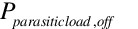 = off-cycle parasitic
electric load (W)
= off-cycle parasitic
electric load (W)
 = HVAC system simulation
time step (hours)
= HVAC system simulation
time step (hours)
Note: All output variables, including off cycle parasitic
electrical power and energy, equal 0 when the desuperheater
heating coil availability schedule equals 0.
Heat
Exchanger Assisted Air Cooling Coil Systems[LINK]
An air-to-air heat exchanger can be used to enhance the
dehumidification performance of a conventional cooling coil.
EnergyPlus has two compound objects to model this scenario: CoilSystem:Cooling:DX:HeatExchangerAssisted
and CoilSystem:Cooling:Water:HeatExchangerAssisted.
The input syntax for these compound objects can be found in
the EnergyPlus Input/Output Reference.
As shown in Figure 161, the air-to-air heat exchanger
pre-conditions the air entering the cooling coil, and reuses
this energy to post-condition the supply air leaving the
cooling coil. This heat exchange process improves the latent
removal performance of the cooling coil by allowing it to
dedicate more of its cooling capacity toward dehumidification
(lower sensible heat ratio).
NOTE: Node naming shown in Figure 161 is representative for
HeatExchanger:AirToAir:SensibleAndLatent.
For HeatExchanger:AirToAir:FlatPlate,
the exhaust air nodes are referred to as ‘secondary air’
nodes. For HeatExchanger:Desiccant:BalancedFlow
(heat exchanger assisted DX coil only), the supply air nodes
are referred to as ‘regeneration air’ nodes and the exhaust
air nodes as ‘process air’ nodes.
The dehumidification performance of cooling coils can be
enhanced using a sensible-only heat exchanger (e.g., heat
pipes, runaround coils, cross-flow heat exchangers). For
example, a CoilSystem:Cooling:DX:HeatExchangerAssisted
object could be used with a HeatExchanger:AirToAir:FlatPlate
object or HeatExchanger:AirToAir:SensibleAndLatent
object with only sensible effectiveness specified (see
resulting psychrometric process in Figure 162). The
dehumidification performance of cooling coils can also be
enhanced using heat exchangers that transfer both sensible and
latent energy (e.g., rotary desiccant heat exchanger). For
example, a CoilSystem:Cooling:DX:HeatExchangerAssisted
object could be used with a HeatExchanger:Desiccant:BalancedFlow
object (see resulting psychrometric process in Figure
163).
Note that while the HeatExchanger:AirToAir:SensibleAndLatent
and HeatExchanger:Desiccant:BalancedFlow
objects can transfer both sensible and latent heat between two
air streams, the HeatExchanger:Desiccant:BalancedFlow
object with appropriate Performance Data Type object is the
proper heat exchanger model to use for the heat exchanger
assisted cooling coil described here. The HeatExchanger:AirToAir:SensibleAndLatent
object should only be used to model the sensible-only heat
exchange case (Figure 162).
Modeling of the heat exchanger assisted cooling coil is
performed by consecutively modeling the air-to-air heat
exchanger and the cooling coil until convergence on a solution
is achieved. The detailed modeling calculations for the
individual components (air-to-air heat exchangers and cooling
coils) are described elsewhere in this document.
Modeling of the heat exchanger assisted cooling coil begins
by initializing the air mass flow rate (based on the air mass
flow rate placed on the compound object’s inlet air node) and
passing this value to the exhaust air inlet node of the
air-to-air heat exchanger. The heat exchanger and cooling coil
are then successively modeled using the calculation routines
specific to the type of heat exchanger and cooling coil
selected. The air temperature exiting the cooling coil is
compared with the air temperature exiting the cooling coil on
the previous modeling iteration for this simulation time step.
Convergence is reached when the change in this air temperature
for successive iterations is within a specified tolerance
(0.0005°C). Consecutive modeling of the heat exchanger and
cooling coil is terminated and a warning message is issued if
the number of modeling iterations exceeds 50.
For the CoilSystem:Cooling:DX:HeatExchangerAssisted
object, heat exchanger operation can be controlled based on
high humidity levels in a zone. By default, the heat exchanger
is assumed to always provide its heat transfer when the
associated DX cooling coil is operating and no humidity
control mechanism is specified. However, the heat exchanger’s
energy transfer may be controlled (i.e., turned on and off)
based on a zone air humidity level using either a humidistat
alone (Figure 164) or a humidistat and a maximum humidity
setpoint manager (Figure 165) depending on the HVAC system
that is utilizing the heat exchanger assisted cooling
coil.
The heat exchanger assisted DX cooling coil may be used
with furnaces or unitary systems located in an air loop (ref.
AirLoopHVAC:Unitary:Furnace:HeatCool
or AirLoopHVAC:UnitaryHeatCool). These system objects have
three options for dehumidification control (None, Multimode,
and CoolReheat). When no dehumidification control is specified
in the furnace or unitary system object (None), the heat
exchanger is always active when the cooling coil is operating.
When multimode or coolreheat dehumidification control is
specified, a humidistat is required as shown in Figure 164.
For the case of multimode dehumidification control, the heat
exchanger is only active when the zone air humidity level is
above the humidistat setpoint (i.e., the system’s cooling coil
can’t meet the latent cooling load when operating without heat
exchanger energy transfer) while the AC system operates to
meet the sensible (dry-bulb cooling thermostat) load. For the
case of coolreheat dehumidification control, the heat
exchanger is always active when the cooling coil operates and
this system tries to meet both the sensible (thermostat) and
latent (humidistat) loads.
The heat exchanger assisted DX cooling coil may also be
used with a DX system located in an air loop (ref.
AirLoopHVAC:UnitaryCoolOnly). This system object also has
three options for dehumidification control (None, Multimode,
and CoolReheat). When no dehumidification control is specified
(None), the heat exchanger is always active when the cooling
coil is operating. When multimode or coolreheat
dehumidification control is specified, a humidistat and a
maximum humidity setpoint manager are required as shown in
Figure 165 (setpoint needs to be placed on the DX system’s
control node). For multimode dehumidification control, the
heat exchanger is only active when the zone humidity levels
are above the humidistat setpoint (i.e., the system’s cooling
coil can’t meet the maximum humidity ratio setpoint when
operating without heat exchanger energy transfer) while the AC
system operates to meet the sensible (dry-bulb cooling
thermostat) load. For coolreheat dehumidification control, the
heat exchanger is always active when the cooling coil operates
and this system tries to meet both the sensible (thermostat)
and latent (humidistat) loads.
When the heat exchanger assisted cooling coil is used with
a furnace or unitary system (ref. AirLoopHVAC:Unitary:Furnace:HeatCool
or AirLoopHVAC:UnitaryHeatCool) or DX system (ref.
AirLoopHVAC:UnitaryCoolOnly) located in an air loop (or DX
system used in an outside air system), an ecomizier function
may be customized as necessary. For economizer control, an
outdoor air controller (ref. Controller:OutdoorAir) is used to
define the economizer control inputs and determine when
economizer mode is active. The heat exchanger (ref.
HeatExchanger:*) object provides an economizer lockout feature
which disables heat recovery any time the economizer is
active. This feature can be turned on and off using the heat
exchanger lockout input. Heat exchanger assisted cooling coils
used with the zone equipment described below disregard this
economizer control feature.
The heat exchanger assisted DX cooling coil may also be
used with the unitary changeover bypass system and the unitary
air-to-air heat pump system (ref. AirLoopHVAC:UnitaryHeatCool:VAVChangeoverBypass
and AirLoopHVAC:UnitaryHeatPump:AirToAir); however, the heat
exchanger is assumed to always provide its heat transfer when
the cooling coil operates and can not be turned on and off
based on a zone air humidity setpoint (ref. Figure 161). Two
zone air conditioners may also use this heat exchanger/coil
assembly model for improved dehumidification. The first type
is the packaged terminal heat pump (ref.
ZoneHVAC:PackagedTerminalHeatPump) where the heat exchanger’s
heat transfer is always active whenever the cooling coil
operates (ref. Figure 161). The second type is the window air
conditioner (ref. ZoneHVAC:WindowAirConditioner) where the
heat exchanger’s heat transfer is always active when the
cooling coil operates and no humidity control mechanism is
specified (ref. Figure 161), or the heat exchanger’s heat
transfer may be controlled based on zone air humidity level
when a humidistat and high humidity setpoint manager are
specified (maximum humidity ratio setpoint must be placed on
the heat exchanger’s exhaust air outlet node). For this case,
the heat exchanger is only active when the zone air humidity
level is above the humidistat setpoint (i.e., the system’s
cooling coil can’t meet the maximum humidity ratio setpoint
when operating without heat exchanger energy transfer) while
only the sensible (dry-bulb cooling thermostat) load is met by
the AC system (ref. Figure 165).
For the CoilSystem:Cooling:Water:HeatExchangerAssisted
object, there is currently no method to enable or disable heat
exchange based on zone air humidity level. Heat exchange will
occur whenever the heat exchanger is available to operate (via
its availability schedule) and a temperature difference exists
between the two air streams.
Kosar, D. 2006. Dehumidification Enhancements, ASHRAE
Journal, Vol. 48, No. 2, February 2006.
http://www.ashrae.org
Kosar, D. et al. 2006. Dehumidification Enhancement of
Direct Expansion Systems Through Component Augmentation of the
Cooling Coil. 15th Symposium on Improving Building
Systems in Hot and Humid Climates, July 24-26, 2006.
http://www.hothumidsymposium.org/
Nimmo, B.G. et al. 1993. DEAC: Desiccant Enhancement of
Cooling-Based Dehumidification. ASHRAE Transactions, Vol.99,
Part 1, Paper number CH-93-4-4, pp. 842-848.
http://www.ashrae.org
Single-Speed
Electric Heat Pump DX Water Heating Coil[LINK]
The input object Coil:WaterHeating:AirToWaterHeatPump
provides a model used in a heat pump water heater (HPWH)
consisting of a water heater tank (e.g., WaterHeater:Mixed), a
direct expansion (DX) “coil” (i.e., an air-to-water DX
compression system which includes a water heating coil, air
coil, compressor, and water pump), and a fan to provide air
flow across the air coil associated with the DX compression
system. These objects work together to model a system which
heats water using zone air, outdoor air, or a combination of
zone and outdoor air as the primary heat source. The heat pump
water heater (Ref. WaterHeater:HeatPump), water heater tank
(Ref. WaterHeater:Mixed), and fan (Ref. Fan:*) objects are
described elsewhere in this document.
The heat pump water heater DX coil model described here
determines the thermal performance and energy consumption of
the DX compression system, which includes a water heating coil
(condenser), a coil used to extract heat from air
(evaporator), and the compressor. This model also simulates
the performance of a condenser water pump that is assumed to
cycle on and off with the compressor.
Virtually all of the inputs to this DX coil model relate to
its water heating performance and energy consumption. The
air-side cooling capacity of this DX system is derived from
user inputs and some model assumptions. The sensible/latent
cooling capacity split is defined by the user at rated
conditions, and the model adjusts this split at off-rated
conditions.
Model Description[LINK]
The user must input the heating capacity, coefficient of
performance (COP), and the sensible heat ratio (SHR) of the
evaporator coil at rated inlet fluid temperatures and flow
rates that are also specified by the user. The evaporator SHR
should be a “gross” value, excluding any thermal impacts due
to the indoor supply air fan. The user may also input up to
seven performance curves that describe the change in total
water heating capacity and efficiency at off-rated and
part-load conditions.
- Heating capacity modifier curve (function of
temperature)
- Heating capacity modifier curve (function of air flow
fraction)
- Heating capacity modifier curve (function of water flow
fraction)
- Heating COP modifier curve (function of temperature)
- Heating COP modifier curve (function of air flow
fraction)
- Heating COP modifier curve (function of water flow
fraction)
- Part load fraction correlation (function of part load
ratio)
Note: The air dry-bulb or wet-bulb temperature used in the
following curve objects is the inlet air temperature to the
HPWH evaporator coil/fan assembly. If the fan placement
specified in the WaterHeater:HeatPump
compound object is draw-through, then the inlet air
temperature represents the temperature of the air entering the
evaporator coil itself. If blow-through fan placement is
specified, then the inlet air temperature represents air
conditions entering the fan located immediately in front
(upstream) of the evaporator coil.
- The heating capacity as a function of temperature modifier
curve defines the variation in DX coil heating capacity as a
function of inlet fluid (air and water) temperatures. The
curve object may use either a bi-quadratic or cubic form. The
bi-quadratic curve uses inlet air temperature (dry-bulb or
wet-bulb temperature based on the input field Evaporator Air
Temperature Type for Curve Objects) and condenser inlet water
temperature as the independent variables. The cubic curve uses
inlet air (dry-bulb or wet-bulb) temperature as the
independent variable. The curve should be normalized to have
the value of 1.0 at the rating point temperatures specified by
the user.
or
where:
 = dry-bulb or wet-bulb
temperature of the air entering the evaporator coil/fan
assembly based on the Evaporator Air Temperature Type for
Curve Objects specified by the user (°C)
= dry-bulb or wet-bulb
temperature of the air entering the evaporator coil/fan
assembly based on the Evaporator Air Temperature Type for
Curve Objects specified by the user (°C)
 = temperature of the
water entering the DX coil condenser (°C)
= temperature of the
water entering the DX coil condenser (°C)
- The heating capacity as a function of air flow fraction
modifier curve is a quadratic or cubic curve that defines the
variation in DX coil heating capacity as a function of the
ratio of actual air flow rate across the evaporator coil to
the rated evaporator air flow rate (i.e., fraction of full
load air flow rate). When used, the output of this curve
should be normalized to have the value of 1.0 at an air flow
fraction of 1.
or
where:
Note: The actual volumetric air flow rate through the
evaporator coil/fan assembly for any simulation time step
where the compressor is operating must be between 0.00002684
m3/s and .00008056 m3/s per watt of
rated total heating capacity. The simulation will issue a
warning message if this air flow range is exceeded, but the
simulation will continue.
- The heating capacity as a function of water flow fraction
modifier curve is a quadratic or cubic curve that defines the
variation in DX coil heating capacity as a function of the
ratio of actual water flow rate through the condenser to the
rated condenser water flow rate (i.e., fraction of full load
water flow rate). When used, the output of this curve should
be normalized to have the value of 1.0 at a water flow
fraction of 1.
or
where:
- The heating COP as a function of temperature modifier
curve defines the variation in DX coil heating COP as a
function of inlet fluid (air and water) temperatures. The
curve object may use either a bi-quadratic or cubic form. The
bi-quadratic curve uses inlet air temperature (dry-bulb or
wet-bulb temperature based on the input field Evaporator Air
Temperature Type for Curve Objects) and condenser inlet water
temperature as the independent variables. The cubic curve uses
inlet air (dry-bulb or wet-bulb) temperature as the
independent variable. The curve should be normalized to have
the value of 1.0 at the rating point temperatures specified by
the user.
or
- The heating COP as a function of air flow fraction
modifier curve is a quadratic or cubic curve that defines the
variation in DX coil heating COP as a function of the ratio of
actual air flow rate across the evaporator coil to the rated
evaporator air flow rate (i.e., fraction of full load air flow
rate). When used, the output of this curve should be
normalized to have the value of 1.0 at an air flow fraction of
1.
or
- The heating COP as a function of water flow fraction
modifier curve is a quadratic or cubic curve that defines the
variation in DX coil heating COP as a function of the ratio of
actual water flow rate through the condenser to the rated
condenser water flow rate (i.e., fraction of full load water
flow rate). When used, the output of this curve should be
normalized to have the value of 1.0 at a water flow fraction
of 1.
or
- The part load fraction as a function of part load ratio
correlation curve parameterizes the variation of electrical
power input to the heat pump DX coil as a function of the part
load ratio (PLR, heating delivered/steady-state heating
capacity). The part load ratio divided by the part load
fraction yields the runtime fraction of the DX heating coil
for a given simulation time step. The part load fraction
correlation accounts for efficiency losses due to compressor
cycling.
or
where:
The part load fraction correlation should be normalized to
a value of 1.0 when the part load ratio equals 1.0 (i.e., no
efficiency losses when the compressor runs continuously for
the simulation time step). For PLR values between 0 and 1 (0
<= PLR < 1), the following rules apply:
PLF >= 0.7 and PLF >= PLR
If PLF < 0.7 a warning message is issued, the program
resets the PLF value to 0.7, and the simulation proceeds. The
runtime fraction of the coil is defined as PLR/PLF. If PLF
< PLR, then a warning message is issued and the runtime
fraction of the coil is limited to 1.0.
When the part load fraction correlation for a heat pump
water heater DX coil is unknown, the typical part load
fraction correlation for a conventional, single-speed DX
cooling coil (e.g., residential or small commercial unit) may
be used:
PLF = 0.85 + 0.15(PLR)
All seven curves are accessed through EnergyPlus’ built-in
performance curve equation manager (curve:quadratic,
curve:cubic and curve:biquadratic). It is not imperative that
the user utilize all coefficients shown in the equations above
if their performance equation has fewer terms (e.g., if the
user’s part load fraction correlation curve is linear instead
of quadratic, simply enter the values for a and b, and set
coefficient c equal to zero).
Note: If any of the above performance curves are not
specified by the user, the output of that curve is assumed to
be 1 for the entire simulation.
For any simulation time step, the heating capacity of the
heat pump water heater DX coil is calculated as follows:
In a similar fashion, the coefficient of performance for
the DX coil for any simulation time step is calculated using
the following equation:
The electric power for the heat pump water heater DX coil
is then calculated using the water heating capacity and
coefficient of performance calculated above.
where:
 = water heating capacity
at the current operating conditions (W)
= water heating capacity
at the current operating conditions (W)
 = water heating capacity
at rated conditions, user input (W)
= water heating capacity
at rated conditions, user input (W)
 = coefficient of
performance at the current operating conditions (W/W)
= coefficient of
performance at the current operating conditions (W/W)
 = coefficient of
performance at rated conditions, user input (W/W)
= coefficient of
performance at rated conditions, user input (W/W)
 = DX heating coil power
(electricity consumption rate) at the current operating
conditions (W)
= DX heating coil power
(electricity consumption rate) at the current operating
conditions (W)
The heating capacity calculated above may or may not
include the impact of pump heat. For this reason, the user
input Condenser Pump Heat Included in Rated Heating Capacity
and Rated COP is used to determine the total water heating
capacity including pump heat.
where:
 = total water heating
capacity including condenser pump heat (W)
= total water heating
capacity including condenser pump heat (W)
 = condenser water pump
power, user input (W)
= condenser water pump
power, user input (W)
 = fraction of condenser
pump heat to water, user input
= fraction of condenser
pump heat to water, user input
Compressor power (electricity consumption rate) is then
calculated based on two additional inputs provided by the
user. The first input specifies if the condenser pump heat is
included in the rated heating capacity and rated COP. If the
condenser pump heat is included in the rated heating capacity
and COP, then condenser pump power must be subtracted from the
DX heating coil power calculated above to determine the
compressor power.
The second of these inputs specifies if the evaporator fan
power is included in the rated heating COP. If evaporator fan
power is included in the rated COP, then fan power must also
be subtracted from the DX heating coil power to determine the
compressor power as follows:
where:
 = Compressor power
(electric consumption rate) at the current operating
conditions (W)
= Compressor power
(electric consumption rate) at the current operating
conditions (W)
 = Fan power, specified in
Fan:OnOff
object (W)
= Fan power, specified in
Fan:OnOff
object (W)
If fan power is not included in the rated heating COP, then
the calculation of compressor power only includes condenser
pump power and does not involve the fan:
The model assumes that all compressor power is rejected as
heat via the DX heating coil. Therefore, the evaporator total
cooling capacity at the current operating conditions is
determined depending on the user input for pump heat:
where:
 = Total evaporator
cooling capacity at the current operating conditions (W)
= Total evaporator
cooling capacity at the current operating conditions (W)
This evaporator cooling capacity is used to calculate the
air-side performance of the heat pump water heater DX coil.
The sensible heat ratio of the cooling capacity at rated
conditions is specified by the user in the input for this DX
coil object. The calculation of sensible heat ratio at
off-rated conditions uses the ADP/BF approach described for
the DX cooling coil model (Ref. Coil Model – DX Cooling Coil
Model). The exiting air conditions for the HPWH DX coil are
calculated the same way as they are for the DX cooling coil
model (cycling fan, cycling coil). The crankcase heater power
and consumption are also calculated using the same equations
used for the DX cooling coil model.
The runtime fraction of the DX coil compressor is
calculated as the ratio of the compressor part load ratio to
the part load fraction correlation entered by the user. The
part load ratio of the DX coil is determined by the heat pump
water heater compound object (Ref. WaterHeater:HeatPump) and
is used by the DX coil to determine the run time fraction of
the compressor.
Finally, the condenser water outlet temperature is
calculated based on the total water heating capacity of the DX
coil and the actual condenser water mass flow rate.
where:
 = condenser outlet water
temperature when the DX coil is operating (˚C)
= condenser outlet water
temperature when the DX coil is operating (˚C)
 = condenser inlet water
temperature (˚C)
= condenser inlet water
temperature (˚C)
 = specific heat of water
entering the condenser coil (J/kg-C)
= specific heat of water
entering the condenser coil (J/kg-C)
 = actual condenser water
mass flow rate when the coil is operating, defined in the WaterHeater:HeatPump
parent object (kg/s)
= actual condenser water
mass flow rate when the coil is operating, defined in the WaterHeater:HeatPump
parent object (kg/s)
Model Outputs[LINK]
After completing the calculations for heating capacity and
power and the final compressor part load ratio has been
determined, the output (report) variables are calculated as
follows:
where:
tsys = HVAC system simulation time
step, hr
SHR = sensible heat ratio at the current inlet air
conditions and air flow rate (Ref. Coil Model – DX Cooling
Coil Model, ADP/BF approach)
Pcrankcase= Crankcase heater capacity,
user input (W)
Water
Source Electric DX Air Cooling Coil[LINK]
There are two objects for water-to-air heat pumps in
cooling mode: Coil:Cooling:WaterToAirHeatPump:EquationFit
and Coil:Cooling:WaterToAirHeatPump:ParameterEstimation.
These are described elsewhere.
Water
Source Electric Heat Pump DX Air Heating Coil[LINK]
There are two objects for water-to-air heat pumps in
heating mode: Coil:Heating:WaterToAirHeatPump:EquationFit
and Coil:Heating:WaterToAirHeatPump:ParameterEstimation.
These are described elsewhere.
Steam-Based Air Heating
Coil[LINK]
The steam coils are included in the discussion on steam
loops, see: Steam To Air Heat Exchanger.
Variable
Refrigerant Flow Cooling Coil[LINK]
The variable refrigerant flow (VRF) DX cooling coil model
is identical to the single-speed DX cooling coil model (Ref.
Coil:Cooling:DX:SingleSpeed) when the compressor operates at
it’s maximum speed. The calculations used when the VRF heat
pump operates at part-load are slightly different than the
single-speed DX cooling coil model. For this reason, an
adaptation of the single-speed DX cooling coil model is used
to model the variable-speed compression system used in the VRF
model. The difference in model calculations occur when the VRF
DX cooling coil’s electronic expansion device reduces
refrigerant flow through the cooling coil. When the
refrigerant flow is reduced, the coil’s apparatus dew point
(ADP) temperature changes, as well as the coil’s sensible heat
ratio (SHR). Since the single-speed DX cooling coil model is
able to determine the ADP and SHR of a cooling coil at various
operating conditions, this same model concept will be used to
determine the ADP and SHR of the variable refrigerant flow DX
cooling coil.
Model Description[LINK]
The user must input the total cooling capacity and the
volumetric air flow rate across the cooling coil at rated
conditions. The capacity input should be “gross” values,
excluding any thermal or energy impacts due to the indoor
supply air fan. The rated volumetric air flow should be
between 0.00004027 m3/s and 0.00006041
m3/s per watt of rated total cooling capacity (300
– 450 cfm/ton).
The user is required to input a performance curve in the
heat pump object (ref: AirConditioner:
VariableRefrigerantFlow) that describes the change in total
cooling capacity at various operating conditions (i.e. at
cooling coil inlet air wet-bulb and condenser entering air
dry-bulb temperatures different than those used to define
total capacity). Each DX cooling coil uses two Cooling
Capacity Ratio Modifier curves to define the DX cooling coil
performance. The first curve defines the full load performance
solely as a function of indoor wet-bulb temperature or uses
both indoor wet-bulb temperature and outdoor dry-bulb
temperature as the independent variables. The specific
performance curves are:
Total cooling capacity modifier curve (function of
temperature)
Total cooling capacity modifier curve (function of flow
fractionl)
- The total cooling capacity modifier curve (function of
temperature) defines the performance of the DX cooling coil as
a function of operating conditions. These operating conditions
may be specified as either a linear, quadratic or cubic
equation using coil entering air wet-bulb temperature as the
independent variable or as a biquadratic equation using both
coil entering air wet-bulb temperature and outdoor dry-bulb
temperuate as the independent variables. Since the variable
refrigerant flow system modulates the compressor speed to
serve the individual cooling coils, the single indpendent
variable equation is likely to be sufficient to define the DX
cooling coil performance. However, if other more accurate
information is available, a biquadratic curve using two
independent variables may be used. The output of this curve is
multiplied by the rated total cooling capacity to give the
total cooling capacity at the specific entering air
temperatures at which the DX coil unit is operating (i.e., at
temperatures different from the rating point
temperatures).
where
= wet-bulb temperature of
the air entering the cooling coil, °C
= dry-bulb temperature of
the air entering an air-cooled condenser
or wet-bulb temperature of the air entering an
evaporative-cooled condenser, °C
The total cooling capacity modifier curve (function of flow
fraction) is a linear, quadratic, or cubic curve with the
independent variable being the ratio of the actual air flow
rate across the cooling coil to the rated air flow rate (i.e.,
fraction of full load flow). The output of this curve is
multiplied by the operating (modulated) total cooling capacity
and the total cooling capacity modifier curve (function of
temperature) to give the total cooling capacity at the
specific temperature and air flow conditions at which the DX
unit is operating. The cubic form of the equation is:
where
Note: The actual volumetric air flow rate
through the cooling coil for any simulation time step where
the DX unit is operating must be between 0.00002684
m3/s and .00006713 m3/s per watt of
rated total cooling capacity (200 - 500 cfm/ton). The
simulation will issue a warning message if this air flow range
is exceeded.
For any simulation time step, the total (gross) cooling
capacity of the DX unit is calculated as follows:
where
= Total available cooling
capacity, W
 = Total reference (rated)
cooling capacity, W
= Total reference (rated)
cooling capacity, W
In addition to calculating the total cooling capacity
provided by the DX cooling coil, it is important to properly
determine the break down of total cooling capacity into its
sensible (temperature) and latent (dehumidification)
components. The model computes the sensible/ latent split
using the SHR and ADP/BF approach (Carrier et al. 1959). When
the DX coil model is initially called during an EnergyPlus
simulation, the rated total capacity and rated SHR are used to
calculate the coil bypass factor (BF) at rated conditions. The
rated total capacity and rated SHR are first used to determine
the ratio of change in air humidity ratio to air dry-bulb
temperature:
where
ωin~~= humidity ratio of the air
entering the cooling coil at rated conditions, kg/kg
ωout~~= humidity ratio of the air
leaving the cooling coil at rated conditions, kg/kg
Tdb,in~~= dry-bulb temperature of the
air entering the cooling coil at rated conditions, °C
Tdb,out~~= dry-bulb temperature of the
air leaving the cooling coil at rated conditions, °C
Along with the rated entering air conditions, the algorithm
then searches along the saturation curve of the psychrometric
chart until the slope of the line between the point on the
saturation curve and the inlet air conditions matches
SlopeRated. Once this point, the apparatus dew point,
is found on the saturation curve the coil bypass factor at
rated conditions is calculated as follows:
where
hout,rated ~~= enthalpy of the air
leaving the cooling coil at rated conditions, J/kg
hin,rated ~~= enthalpy of the air
entering the cooling coil at rated conditions, J/kg
hADP ~~= enthalpy of saturated air at
the coil apparatus dew point, J/kg
The coil bypass factor is analogous to the
“ineffectiveness” (1-ε) of a heat exchanger, and can be
described in terms of the number of transfer of unit
(NTU).
For a given coil geometry, the bypass factor is only a
function of air mass flow rate. The model calculates the
parameter Ao in the equation above based on
BFrated and the rated air mass flow rate. With
Ao known, the coil BF can be determined for
non-rated air flow rates.
For each simulation time step when the DX cooling coil
operates, the total cooling capacity and coil bypass factor at
the actual operating conditions are calculated. The coil
bypass factor is used to calculate the operating sensible heat
ratio (SHR) of the cooling coil using the following equations.
Here is where the differnce in models occur for the VRF DX
cooling coil and single-speed DX cooling coil. The original
coil model (ref: Coil:Cooling:DX:SingleSpeed) calculates the
full load outlet air enthalpy and, considering the bypass
factor, finds the coil surface temperture (hADP) at
full load (i.e., PLR = 1). Conversely, the VRF coil model
modulates refrigerant flow to the VRF DX cooling coil which is
why this model uses the full load coil capacity multipled by
the part-load ratio (the modulated refrigerant flow). The
effectively finds the coil surface temperature for a variable
refrigerant flow DX cooling coil and the operating sensible
heat ratio (SHR) can be calculated.
 ; single-speed DX coil
model (hADP1 in figure below),
; single-speed DX coil
model (hADP1 in figure below),
 ; variable refrigerant
flow DX coil model
; variable refrigerant
flow DX coil model
where
= enthalpy of the air
entering the cooling coil, J/kg
= enthalpy of air at the
apparatus dew point condition, J/kg
= enthalpy of air at the
entering coil dry-bulb temperature and humidity ratio at ADP,
J/kg
= air mass flow rate,
kg/s
With the SHR for the coil at the current operating
conditions, the properties of the air leaving the cooling coil
are calculated using the following equations:
where
= enthalpy of the air
leaving the cooling coil, J/kg
= enthalpy of air at the
entering coil dry-bulb temperature and leaving air humidity
ratio, J/kg
= leaving air humidity
ratio, kg/kg
= leaving air dry-bulb
temperature, °C
PsyWFnTdbH = EnergyPlus psychrometric function,
returns humidity ratio given dry-bulb temperature and
enthalpy
PsyTdbFnHW = EnergyPlus psychrometric function,
returns dry-bulb temperature given enthalpy and humidity
ratio
The following figure shows this process on a psychrometric
chart. This variable refrigerant flow DX cooling coil model
follows the dotted process line from hin towards
the outlet air enthalpy (the clear circles, ο) based on the
modulated refrigerant flow (PLR). The coil surface temperature
(ADP, apparatus dew point) is found by drawing a straight line
through these points. The process line from hin to
hADP1 represents the full load (PLR=1). This would
be what the original DX cooling coil model calculates. At this
point the sensible heat ratio is at the design point (assuming
hin is the rating point and the coil operates at
the rated air mass flow rate). As the coil load is reduced,
the refrigerant flow rate is restricted and the outlet air
condition rides up the dotted line. The outlet air condition
and associated hADP2 is shown for a PLR of 0.7 (for
example purposes only). Here the sensible heat ratio is higher
than that found at full load operation. As the load continues
to reduce, the refrigerant flow rate continues to throttle
back and there comes a point where the coil’s ADP is equal to
the inlet air dew point temperature (hADP3). At
this point, and for all other PLR’s less than this value, the
coil surface becomes dry (at PLR=0.4 in this example) and the
coil’s sensible heat ratio = 1. Between this PLR and PLR=0,
the coil outlet air condition follows the dotted line back
towards Hin.
Dry Coil Conditions[LINK]
If the model determines that the cooling coil is dry
(ωin < ωADP), then the equation for
total cooling capacity is invalid since it is a function of
entering wet-bulb temperature. Under dry-coil conditions, coil
performance is a function of dry-bulb temperature rather than
wet-bulb temperature. In this case, the model recalculates the
performance of the DX cooling unit using the calculation
procedure described above but with ω~in
=ωdry,~where ωdryis the inlet air
humidity ratio at the coil dry-out point (SHR = 1.0).
Condenser
Options: Air Cooled vs. Evaporative Cooled[LINK]
As described previously, this model can simulate the
performance of air-cooled or evaporative-cooled DX air
conditioners. The choice of condenser type impacts the air
dry-bulb temperature entering the heat pump’s condenser.
Although the actual input for the selection is contained in
the variable refrigerant flow air conditioner object, the
calculations are repeated here to aid the user in
understanding the condenser option choices. The following
paragraphs describe three modeling options.
If the user wants to model an air-cooled condenser, they
should simply specify AirCooled in the field Condenser Type.
In this case, the Total Cooling Capacity Modifier Curve
(function of temperature) and the Energy Input Ratio Modifier
Curve (function of temperature) will utilize the outdoor
dry-bulb temperature.
If the user wishes to model an evaporative-cooled condenser
AND they have performance curves that are a function of the
wet-bulb temperature of air entering the condenser coil, then
the user should specify Condenser Type = EvapCooled and the
evaporative condenser effectiveness value should be entered as
1.0. In this case, the Total Cooling Capacity Modifier Curve
(function of temperature) will utilize the outdoor wet-bulb
temperature.
If the user wishes to model an air-cooled condenser that
has evaporative media placed in front of it to cool the air
entering the condenser coil, then the user should specify
Condenser Type = EvapCooled. The user must also enter the
appropriate evaporative effectiveness for the media. In this
case, the Total Cooling Capacity Modifier Curve (function of
temperature) and the Energy Input Ratio Modifier Curve
(function of temperature) will utilize the condenser inlet air
temperature as calculated below:
where
Tc,i~~= the temperature of the air
entering the condenser coil, °C
Twb,o~~= the wet-bulb temperature of
the outdoor air, °C
Tdb,o~~= the dry-bulb temperature of
the outdoor air, °C
The Total Cooling Capacity Modifier Curve (function of
temperature) and the Energy Input Ratio Modifier Curve
(function of temperature) input fields for the variable
refrigerant flow air conditioner object should reference
performance curves that are a function of outdoor dry-bulb
temperature. Be aware that the evaporative media will
significantly reduce the dry-bulb temperature of the air
entering the condenser coil, so the Total Cooling Capacity and
EIR Modifier Curves must be valid for the expected range of
dry-bulb temperatures that will be entering the condenser
coil.
Condenser Inlet Air
Temperature[LINK]
The air temperature entering the outdoor condenser is based
on the weather data used during a simulation. This temperature
is either taken directly from the weather data, or can be
adjusted based on the height of the outdoor condenser. The
input for Condenser Air Inlet Node Name can be used to control
this optional feature. If this input is left blank, the air
temperature entering the condenser is based solely on the
weather data. If this input is not blank, then the node name
specified must also be listed in an Outside Air Node or
Outside Air Inlet Node List object. When the node name is
listed in an Outside Air Inlet Node List object, the air
temperature entering the condenser is based solely on the
weather data. When the node name is listed in an Outside Air
Node object, the height of the node determines the air
temperature entering the outdoor condenser (see description of
Local Outdoor Air Temperature Calculation in the Atmospheric
Variation section of this document for further details).
Supply
Air Fan Control: Cycling vs. Continuous[LINK]
One of the inputs to the variable refrigerant flow terminal
unit model is the supply air fan operation mode: cycling fan,
cycling compressor or continuous fan, cycling compressor. The
mode specified in the terminal unit object is passed to the DX
cooling coil for use in the model calculations. The first
operation mode is frequently referred to as “AUTO fan”, where
the compressor(s) and supply air fan operate in unison to meet
the zone cooling load, and cycle off together when the cooling
load has been met. The second operation mode is often referred
to as “fan ON”, where the compressor(s) cycle on and off to
meet the zone cooling load but the supply air fan operates
continuously regardless of compressor operation.
The fan operation mode schedule value determines the fan
operation mode for each time step throughout the simulation. A
fan operation mode schedule value of 0 specifies AUTO fan mode
operation while values other than 0 specify fan ON operation.
The use of a schedule allows the fan operation mode to change
based on time-of-day or with changes in season.
The EnergyPlus methodology for determining the impact that
HVAC equipment has on an air stream is to calculate the mass
flow rate and air properties (e.g., enthalpy, dry-bulb
temperature, humidity ratio) exiting the equipment. These
exiting conditions are passed along as inlet conditions to the
next component model in the air stream. Eventually the flow
rate and properties of the air being supplied to the
conditioned zone are used in the zone energy balance to
determine the resulting zone air temperature and humidity
ratio.
With this methodology, the determination of the air mass
flow rate and air properties for the two different supply air
fan operation modes is slightly different. For the case of
cycling fan/cycling compressor, the conditions of the air
leaving the cooling coil are the steady-state values
calculated using the equations described above. However the
air mass flow rate passed along to the next component (and
eventually to the conditioned zone) is the average air mass
flow rate for the system simulation time step.
For the case of continuous fan/cycling compressor, the air
mass flow rate is constant. However, the air properties
leaving the cooling coil are calculated as the average
conditions during the system simulation time step. The model
assumes that the exiting air conditions are the steady-state
values calculated using the equations described above when the
heat pump operates. For the remainder of the system simulation
time step, it is assumed that the air exiting the DX coil has
the same properties as the air entering the coil. For this
supply air fan operating strategy, the leaving air properties
are calculated as follows:
Average Air Flow
Calculations[LINK]
The variable refrigerant flow (VRF) terminal unit operates
based on user-specified (or autosized) air flow rates. The VRF
terminal unit’s supply air flow rate during cooling operation
may be different than the supply air flow rate during heating
operation. In addition, the supply air flow rate when no
cooling or heating is required but the supply air fan remains
ON can be different than the air flow rates when cooling or
heating is required. The outside air flow rates can likewise
be different for cooling and heating operating modes. The
model takes these different flow rates into account when
modeling the heat pump, and the average air flow rate for each
simulation time step is reported on the inlet/outlet air nodes
of the various terminal unit components in proportion to the
calculated cycling ratio of the coil.
The average supply air and outdoor air mass flow rates
through the heat pump for the HVAC simulation time step are
calculated based on the cycling ratio of the DX cooling coil
or heating coil (whichever coil is operating) as follows:
where:
 = average supply air mass
flow rate during the time step, kg/s
= average supply air mass
flow rate during the time step, kg/s
 = supply air mass flow
rate when the coil is ON, kg/s
= supply air mass flow
rate when the coil is ON, kg/s
CyclingRatio = cycling ratio of the coil (heating
or cooling)
 = supply air mass flow
rate when the coil is OFF, kg/s
= supply air mass flow
rate when the coil is OFF, kg/s
 = average outside air
mass flow rate during the time step, kg/s
= average outside air
mass flow rate during the time step, kg/s
 = average outside air
mass flow rate when the coil is ON, kg/s
= average outside air
mass flow rate when the coil is ON, kg/s
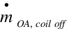 = average outside air
mass flow rate when the coil is OFF, kg/s
= average outside air
mass flow rate when the coil is OFF, kg/s
The supply air and outside air flow rates when the DX
cooling or DX heating coil is ON are specified by the user
(e.g., supply air volumetric flow rate during cooling
operation, supply air volumetric flow rate during heating
operation, outside air volumetric air flow rate during cooling
operation, and outside air volumetric air flow rate during
heating operation) and are converted from volumetric to mass
flow rate. If the user has specified cycling fan operation,
then the supply air and outside air mass flow rates when the
coil is OFF are zero. If the user has specified constant fan
operation, then the user-defined air flow rates when no
cooling or heating is needed are used when the coil is
OFF.
There is one special case. If the user has specified
constant fan operation and they specify that the supply air
volumetric flow rate when no cooling or heating is needed is
zero (or field is left blank), then the model assumes that the
supply air and outside air mass flow rates when the coil is
OFF are equal to the corresponding air mass flow rates when
the coil was last operating (ON).
Variable
Refrigerant Flow Heating Coil[LINK]
The variable refrigerant flow (VRF) DX heating coil model
uses performance information at rated conditions along with
performance curves for variations in total capacity, energy
input ratio and part load fraction to determine performance at
part-load conditions. The impacts of defrost operation is
modeled based a combination of user inputs and empirical
models taken from the air-to-air heat pump algorithms in
DOE-2.1E. The VRF DX heating coil model is very similar to the
DX heating coil model used in the single-speed heat pump. The
only difference being that the energy performance curves were
moved to the parent object (Ref.
AirConditioner:VariableRefrigerantFlow). See the DX Heating
Coil model description for further details.
Variable
Speed Water to Air Heat Pump (Heating & Cooling)[LINK]
Coil:Heating:WaterToAirHeatPump:VariableSpeedEquationFit[LINK]
A Variable Speed Water Source Heat Pump (let’s call it VS
WSHP) has a system control which dictates the refrigerant flow
rate, the design unit supply airflow and the required water
flow rate at each compressor speed. The air and water flow
rates are usually a function of the compressor speed.
Refrigerant mass flow rate is a function of compressor speed
as well as entering water temperature and indoor dry bulb or
wet bulb. The control system adjusts the equipment capacity
based on zone temperature measurements relative to the
thermostat set point. The control logic determines what
compressor speed is required to control to the zone
temperature requirement in response to increased or decreased
capacity (heating or cooling load). The compressor, fan and
pump speeds are not discrete values and can be considered to
vary infinitesimally between the minimum and maximum
compressor speed. At the minimum compressor speed (which is
different for heating and cooling), for a continuous fan, the
supply airflow is fixed and the unit will have to cycle for
reduced part loads below this point. For a cycling fan, the
fan will cycle with the compressor.
Present EnergyPlus is capable of modeling multiple-speed DX
air-to-air coils. The number of speed levels is up to four. In
some cases, four sets of performance curves are not sufficient
to include all the information for a variable speed equipment.
There is a need to expand the space for containing more
performance curves. Here, we expand the number of speed levels
and the corresponding curve sets up to ten. The number of
speed levels is selectable by the user. The user can provide
speed levels at any number from 2 to 10. In any case, our
model would just do linear interpolation between neighboring
speeds. The more curves, the more accurate. Furthermore, using
linear interpolation and inputting air and water flow rates at
individual speed levels facilitates arbitrary relationships of
flow rates as a function of the compressor speed level.
This model (object name
Coil:Heating:WaterToAirHeatPump:VariableSpeedEquationFit)
simulates the performance of a variable-speed water-to-air
heat pump with heating capability. It fits in the parent
objects of AirLoopHVAC:UnitaryHeatPump:WaterToAir
and ZoneHVAC:WaterToAirHeatPump.
The rated conditions for obtaining the Reference Unit total
heating capacities and COPs are indoor dry-bulb temperature at
21.1 ˚C (70 ˚F) and the source side entering water temperature
at 21.1 ˚C (70 ˚F).
Model Description[LINK]
The Coil:Heating:WaterToAirHeatPump:VariableSpeedEquationFit
object is modeled in a manner similar to the multi-speed DX
heating coil model (Ref. Coil:Heating:DX:MultiSpeed). Of
course, rather than referencing an air source evaporator or
defrost object, the new coil object references to the water
loop, and has the entering water temperature in place of the
indoor air entering dry bulb temperature.
It shall be noted for the capacity and flow rate inputs,
three fields are autosizable, which are Rated Heating Capacity
at the Selected Nominal Speed Level (Numeric Field 3), Rated
Volumetric Air Flow Rate (Numeric Field 4) and Rated
Volumetric Water Flow Rate (Numeric Field 5). They are used to
scale the performances of a specific unit and correlate with
the actual loop flows. Except these three fields, all other
capacity and flow rate inputs at individual speed levels
should be directly obtained from Reference Unit catalog data,
specific to an actual unit.
The Rated Heating Capacity at Selected Nominal Speed Level
contains the rated capacity to match the building heating load
at the design day. The rated heating capacity is used to
determine a capacity scaling factor, as compared to the
Reference Unit capacity at the nominal speed level.
And then, this scaling factor is used to determine
capacities at rated conditions for other speed levels, as
below:
The Rated Volumetric Air Flow Rate is used to determine an
internal scaling factor, and calculate the air flow rates in
the parent objects, as follows:
And the loop volumetric air flow rates at various speed
levels in the parent objects are calculated as below:
If the volumetric air flow rate at one speed level is
higher than the flow rate allowed by the fan in the parent
object, the flow rate will be set back to the fan flow
rate.
This Rated Volumetric Water Flow Rate is used to determine
an internal scaling factor, and calculate the loop water flow
rates.
And the required volumetric water flow rates in the parent
objects are calculated as below,
The required volumetric water flow rate as above should be
restricted by the pump in the water loop.
If  and
and  equal unity, the loop flow rates
become the design flow rates of the Reference Unit (after
scaled by the rated heating capacity). The Rated Volumetric
Air Flow Rate and Rated Volumetric Water Flow Rate are
introduced here to correlate with the actual flow rates in the
air and water loops, in case that these differ from the design
specification. Certainly, it is recommended that the Rated
Volumetric Air Flow Rate and Rated Volumetric Water Flow Rate
are selected in the way that
equal unity, the loop flow rates
become the design flow rates of the Reference Unit (after
scaled by the rated heating capacity). The Rated Volumetric
Air Flow Rate and Rated Volumetric Water Flow Rate are
introduced here to correlate with the actual flow rates in the
air and water loops, in case that these differ from the design
specification. Certainly, it is recommended that the Rated
Volumetric Air Flow Rate and Rated Volumetric Water Flow Rate
are selected in the way that  and
and  are unity, so as to get
more accurate results from the performance curves.
are unity, so as to get
more accurate results from the performance curves.
Performance curves:
This object includes 7 curve objects at each individual
speed level.
Total heating capacity modifier curve (function of
temperature).
Total heating capacity modifier curve (function of air
flow fraction).
Total heating capacity modifier curve (function of
water flow fraction).
Energy input ratio (EIR) modifier curve (function of
temperature).
Energy input ratio (EIR) modifier curve (function of
air flow fraction).
Energy input ratio (EIR) modifier curve (function of
water flow fraction).
Recoverable heat modifier as a function of indoor air
dry-bulb and water entering temperatures.
Curves 3) and 6) are new curves as compared to those used
for Multi-Speed Electric DX Air Heating Coil, as to correlate
the change in water flow rate at the speed. The flow fraction
modifier curves are used as a placeholder, to account for
off-design flow rates if needed. If the manufacturer doesn’t
provide off-design performances, we can simply use a default
modification multiplier of 1.0.
At the lowest speed, there will be one additional
performance curve to account for the part-load condition,
i.e.
Part load fraction correlation (function of part load
ratio)
Total heating capacity modifier curve (function of
temperature)
The total heating capacity modifier as a function of
temperature curve (CAP-FT) is a biquadratic curve with two
independent variables: dry-bulb temperature of the air
entering the heating coil and the VS WSHP’s entering water
temperature. The output of this curve is multiplied by the
rated total heating capacity at the speed, to give the total
heating capacity at the specific entering air and water
temperatures at which the WSHP unit is operating (i.e., at
temperatures different from the rating point
temperatures).
where
DBi = dry-bulb temperature of the air entering
the heating coil, °C
EWT = entering water temperature, °C
a-f = regression curve-fit coefficients
- Total heating capacity modifier curve (function of air
flow fraction)
where
ffa = actual air mass flow rate/design air mass
flow rate, at one speed level;
a-d = regression curve-fit coefficients, if no data
available for the correction, the user can simply put a = 1.0,
and the other coefficients as 0.0.
- Total heating capacity modifier curve (function of water
flow fraction)
where
ffw = actual water mass flow rate/design water
mass flow rate, at one speed level;
a-d = regression curve-fit coefficients, if no data
available for the correction, the user can simply put a = 1.0,
and the other coefficients as 0.0.
- Energy input ratio (EIR) modifier curve (function of
temperature)
The energy input ratio modifier curve as a function of
temperature (EIR-FT) is a biquadratic curve with two
independent variables: dry-bulb temperature of the air
entering the heating coil and the WSHP’s entering water
temperature. The output of this curve is multiplied by the
rated EIR at the speed (inverse of the rated COP), to give the
EIR at the specific entering air and water temperatures at
which the WSHP coil unit is operating (i.e., at temperatures
different from the rating point temperatures).
where
DBi = dry-bulb temperature of the air entering
the heating coil, °C
EWT = entering water temperature, °C
a-f = regression curve fit coefficients.
- Energy input ratio (EIR) modifier curve (function of air
flow fraction)
where
a-d = regression curve-fit coefficients, if no data
available for correction, the user can simply put a = 1.0, and
the other coefficients as 0.0.
- Energy input ratio (EIR) modifier curve (function of water
flow fraction)
where
a-d = regression curve fit coefficients, if no data
available for the correction, the user can simply put a = 1.0,
and the other coefficients as 0.0.
- Recoverable heat modifier as a function of indoor dry-bulb
and water entering temperatures.
Recoverable heat modifier function accounts for the
recoverable waste heat at the condensing side, as a fraction
to the input power. This part of heat doesn’t added to the
supply side.
where
a-f = regression curve-fit coefficients.
- Part load fraction correlation (function of part load
ratio)
This field defines the name of a quadratic or cubic
performance curve (Ref: Performance Curves) that parameterizes
the variation of electrical power input to the unit as a
function of the part load ratio (PLR, heating
load/steady-state heating capacity for Speed 1),
And
RTF = (PLR/PartLoadFrac) = runtime fraction of the heating
coil
The part load fraction (PLF) correlation accounts for
efficiency losses due to compressor cycling. The part load
fraction correlation should be normalized to a value of 1.0
when the part load ratio equals 1.0 (i.e., no efficiency
losses when the compressor runs continuously for the
simulation timestep). For PLR values between 0 and 1 (0 <=
PLR < 1), the following rules apply:
PLF >= 0.7 and PLF >= PLR
If PLF < 0.7, the program resets the PLF value to 0.7,
and the simulation proceeds. The runtime fraction of the coil
is defined as PLR/PLF. If PLF < PLR, the runtime fraction
of the coil is limited to 1.0. A typical part load fraction
correlation would be:
If the user wishes to model no efficiency degradation due
to compressor cycling, the part load fraction correlation
should be defined as follows:
Lowest Speed Operation:
The lowest speed operation of the VS WSHP is similar to the
single speed DX heating coil. The total (gross) heating
capacity of the WSHP unit is calculated as follows:
 **
**
And the EIR is calculated as:
And the power consumption including the compressor and
accessories (not including pump and indoor fan powers) is,
The waste heat generated by this coil object is calculated
as:
where
 = waste heat fraction of
the energy input at Speed 1, from the Reference Unit data.
= waste heat fraction of
the energy input at Speed 1, from the Reference Unit data.
The total amount of heat absorbed by the evaporator is
calculated as:
The fraction of the actual air mass flow to the design air
mass flow rate is calculated:
The fraction of the actual water mass flow to the design
water mass flow rate is calculated:
 **
**
Higher Speed Operation:
At the speed level between the lowest and the highest,
there is no part-load loss. A parameter of speed ratio
(SpeedRatio) is used to define the capacity partition between
Speed x-1 and Speed x.
The design air and water flow rate at the speed ratio are
given as following:
And the fractions of air flow and water flow are given:
 =
=  = actual air mass flow
rate/DesignAirFlowRateSpeedRatio
= actual air mass flow
rate/DesignAirFlowRateSpeedRatio
 =
=  = actual water mass flow
rate/DesignWaterFlowRateSpeedRatio
= actual water mass flow
rate/DesignWaterFlowRateSpeedRatio
The total heating capacities and EIRs at Speed x-1 and
Speed x are given:
 **
**
The total heating capacity at the corresponding speed ratio
is:
And the power consumption is
The waste heat generated by this coil object is calculated
as:
 **
**
The total amount of heat absorbed by the evaporator is
calculated as:
At last,
If the speed reaches the highest level, the speed ratio
becomes 1.0, and Speed x represents the highest speed.
Coil:Cooling:WaterToAirHeatPump:VariableSpeedEquationFit[LINK]
This model (object name
Coil:Cooling:WaterToAirHeatPump:VariableSpeedEquationFit)
simulates the performance of an variable-speed water-to-air
heat pump with cooling capability. It fits in the parent
objects of AirLoopHVAC:UnitaryHeatPump:WaterToAir
and ZoneHVAC:WaterToAirHeatPump.
It has the same logic for varying the compressor, indoor fan
and pump speeds as the Coil:Heating:WaterToAirHeatPump:VariableSpeedEquationFit
object. The rated conditions for obtaining the capacities,
COPs and SHR are indoor dry-bulb temperature at 26.67 ˚C (80
˚F), wet bulb temperature at 19.44 ˚C (67 ˚F), and the source
side entering water temperature at 29.4 ˚C (85 ˚F).
Variable-speed cooling coils lead to varied
dehumidification behaviors, that the Bypass Factor (BF) is not
only dependent on the indoor air flow rate, but also on the
refrigerant mass flow rate, i.e. the compressor speed. It is
necessary to assess the BF approach for single-speed DX coil,
to be used for the variable-speed systems.
The DOE/ORNL Heat Pump Design Model (HPDM) is a steady-state vapor compression equipment simulation model, which is able to simulate the performance of a VS WSHP system. We ran a calibrated HPDM model to produce performance data of a 2.5-ton, VS WSHP unit in space cooling mode. We ran the model to get the total cooling capacities and SHRs, by specifying the EWT at 65 ˚F, indoor air DB at 80 ˚F and relative humidity at 0.5, and then varying the indoor air flow rate from 400 scfm to 1000 scfm, the compressor speed from 30 HZ to 90 HZ in a 7×7 matrix. Based on the performance results, we used EES (Engineering Equation Solver) to back-calculate the corresponding BF factors and the A~o~ (effective coil surface area) parameters, using the BF equations for the single speed DX cooling coil in EnergyPlus Engineering Reference.
And then, we plotted the resultant A~o~ as a function of indoor air flow rate and compressor speed, as below:
As indicated in the two figures above, the compressor speed
is a significant factor impacting the Ao parameter
and the BF factor. So, the current BF factor approach should
be upgraded to accommodate variable-speed cooling coils.
As shown in the Ao figure, we can almost assume
that the Ao parameter mainly depends on the
compressor speed. And thus, for enhancing the VS WSHP model,
in the IDF file, we need to input SHRs at individual
compressor speeds (this is similar to the current multi-speed
DX cooling coil). And then, within the VS WSHP module, we
calculate the Ao parameter specific to each
compressor speed at the design air flow rates, and then do
linear interpolation of Ao between neighboring
compressor speeds. For calculating SHRs in energy simulations,
we first calculate the Ao parameter related to the
actual compressor speed, and then use the simulated
Ao parameter in the original BF correlation to
correlate effect of the varied indoor air flow rate.
Model Description[LINK]
The Coil:Cooling:WaterToAirHeatPump:VariableSpeedEquationFit
object is modeled in a manner similar to the multiple-speed DX
cooling coil model (Ref. Coil:Cooling:DX:MultiSpeed). Of
course, rather than referencing an air-cooled condenser, the
new coil object references the water loop, and have the water
entering temperature in place of the condenser air entering
dry bulb temperature.
It shall be noted for the total cooling capacity and flow
rate inputs, three fields are autosizable, which are Rated
Total Cooling Capacity (Numeric Field 3) at Selected Nominal
Speed Level, Rated Volumetric Air Flow Rate (Numeric Field 4)
and Rated Volumetric Water Flow Rate (Numeric Field 5). They
are used to scale the performances of an actual unit and
correlate with the actual loop flows. Except the three fields,
all other total cooling capacity and flow rate inputs at
individual speed levels should be directly obtained from
Reference Unit catalog data, specific to an actual unit.
The Rated Total Cooling Capacity at Selected Nominal Speed
Level contains the rated total cooling capacity to match the
building sensible or latent cooling load. The rated cooling
capacity is used to determine a capacity scaling factor, as
compared to the Reference Unit catalog capacity at the nominal
speed level.
And then, this scaling factor is used to determine
capacities at rated condition for other speed levels, as
below,
The Rated Volumetric Air Flow Rate is used to determine an
internal scaling factor, and calculate the air flow rates in
the parent objects, as follows:
And the loop volumetric air flow rates in the parent
objects are calculated as below,
If the volumetric air flow rate at one speed level is
higher than the flow rate allowed by the fan in the parent
object, the flow rate will be set back to the fan flow
rate.
This Rated Volumetric Water Flow Rate is used to determine
an internal scaling factor, and calculate the loop water flow
rates.
And the required volumetric water flow rates in the parent
objects are calculated as below,
The required volumetric water flow rate as above is
restricted by the pump in the parent object.
If  and
and  are equal to unity, the loop flow
rates become the design flow rates of the original unit (after
scaled by the rated total cooling capacity). The Rated
Volumetric Air Flow Rate and Rated Volumetric Water Flow Rate
are introduced here to correlate with the actual flow rates in
the air and water loops, in case that these differ from the
design specifications. Certainly, it is recommended that the
Rated Volumetric Air Flow Rate and Rated Volumetric Water Flow
Rate are selected in the way that
are equal to unity, the loop flow
rates become the design flow rates of the original unit (after
scaled by the rated total cooling capacity). The Rated
Volumetric Air Flow Rate and Rated Volumetric Water Flow Rate
are introduced here to correlate with the actual flow rates in
the air and water loops, in case that these differ from the
design specifications. Certainly, it is recommended that the
Rated Volumetric Air Flow Rate and Rated Volumetric Water Flow
Rate are selected in the way that  and
and  are unity, so as to get more
accurate results from the performance curves.
are unity, so as to get more
accurate results from the performance curves.
Performance Curves:
This object includes 7 curve objects at each individual
speed level.
Total cooling capacity modifier curve (function of
temperature)
Total cooling capacity modifier curve (function of air
flow fraction)
Total cooling capacity modifier curve (function of
water flow fraction)
Energy input ratio (EIR) modifier curve (function of
temperature)
Energy input ratio (EIR) modifier curve (function of
air flow fraction)
Energy input ratio (EIR) modifier curve (function of
water flow fraction)
Recoverable heat modifier as a function of indoor air
wet-bulb and water entering temperatures.
Curves 3) and 6) are new curves as compared to those used
for Multi-Speed Electric DX Air Cooling Coil, to correlate the
change in water flow rate at the speed. The flow fraction
modifier curves are used as a placeholder, to account for
off-design flow rates if needed. If the manufacturer doesn’t
provide the off-design performances, we can simply use a
default modification multiplier of 1.0.
At the lowest speed, there will be one additional
performance curve to correlate the part-load condition,
i.e.
8) Part load fraction correlation
(function of part load ratio)
- Total cooling capacity modifier curve (function of
temperature)
The total cooling capacity modifier as a function of
temperature curve (CAP-FT) **is a biquadratic curve with two
independent variables: wet-bulb temperature of the air
entering the cooling coil and the WSHP’s entering water
temperature. The output of this curve is multiplied by the
rated total cooling capacity at the speed, to give the total
cooling capacity at the specific entering air WB and water
temperatures at which the WSHP unit is operating (i.e., at
temperatures different from the rating point
temperatures).
Note: The data used to develop the total cooling capacity
modifier curve (function of temperature) should represent
performance when the cooling coil is ‘wet’ (i.e., coil
providing sensible cooling and at least some
dehumidification). Performance data when the cooling coil is
‘dry’ (i.e., not providing any dehumidification) should not be
included when developing this modifier curve. This model
automatically detects and adjusts for ‘dry coil’
conditions.
where
WBi = wet-bulb temperature of the air entering
the heating coil, °C
EWT = entering water temperature, °C
a-f = regression curve-fit coefficients.
- Total cooling capacity modifier curve (function of air
flow fraction)
The total cooling capacity modifier curve (function of air
flow fraction) is a cubic curve with the independent variable
being the ratio of the actual air flow rate across the cooling
coil to the design air flow rate (i.e., fraction of design
flow at the speed).
where
ffa = actual air mass flow rate/design air mass
flow rate, at one speed level;
a-d = regression curve fit coefficients, if no data for
correction, the user can simply put a = 1.0, and the other
coefficients as 0.0.
- Total cooling capacity modifier curve (function of water
flow fraction)
The total cooling capacity modifier curve (function of
water flow fraction) is a cubic curve with the independent
variable being the ratio of the actual water flow rate across
the water-to-refrigerant heat exchanger to the design water
flow rate (i.e., fraction of design flow at the speed).
where
ffw = actual water mass flow rate/design water
mass flow rate, at one speed level;
a-d = regression curve-fit coefficients, if no data
available for the correction, the user can simply put a = 1.0,
and the other coefficients as 0.0.
- Energy input ratio (EIR) modifier curve (function of
temperature)
The energy input ratio modifier curve as a function of
temperature (EIR-FT) is a biquadratic curve with two
independent variables: wet-bulb temperature of the air
entering the cooling coil and the WSHP’s entering water
temperature. The output of this curve is multiplied by the
rated EIR (inverse of the rated COP) at the speed level, to
give the EIR at the specific entering air and water
temperatures at which the WSHP unit is operating (i.e., at
temperatures different from the rating point
temperatures).

where
WBi = wet-bulb temperature of the air entering
the cooling coil, °C
EWT = entering water temperature, °C
a-f = regression curve fit coefficients
- Energy input ratio (EIR) modifier curve (function of air
flow fraction)
where
a-d = regression curve fit coefficients, if no data
available for correction, the user can simply put a = 1.0, and
the other coefficients as 0.0.
- Energy input ratio (EIR) modifier curve (function of water
flow fraction)
where
a-d = regression curve fit coefficients, if no data
available for correction, the user can simply put a = 1.0, and
the other coefficients as 0.0.
- Recoverable heat modifier as a function of indoor wet-bulb
and water entering temperatures.
Recoverable heat modifier function is to account for the
recoverable heat at the condensing side, as a fraction to the
power input, which doesn’t discharged to the water side.

where
a-f = regression curve fit coefficients
- Part load fraction correlation (function of part load
ratio)
This field defines the name of a quadratic or cubic
performance curve (Ref: Performance Curves) that parameterizes
the variation of electrical power input to the unit as a
function of the part load ratio (PLR, Sensible or Latent
Load/Steady-State Sensible or Latent Capacity for Speed 1).
The description of the part load fraction correlation for the
VS WSHP cooling coil is similar to the VS WSHP heating
coil.
Lowest Speed Operation:
The lowest speed operation of the VS WSHP is similar to the
single speed DX cooling coil. The total (gross) cooling
capacity of the WSHP unit is calculated as follows:
And the EIR is calculated as:
 **
**
And the power consumption excluding the indoor fan and the
water pump is,

Where RTF is the run-time fraction.
The recoverable waste heat is:
And the net heat discharged to the water loop is calculated
as following:
 .
.
At the lowest speed, the dehumidification calculation is
exactly the same as the single speed DX coil. That is to use
the rated SHR and the design air flow rate at the lowest speed
to calculate rated bypass factor of BFrated,1, and
the corresponding effective surface area of Ao,1.
Wh Ao,1 known, the coil BF can be adjusted for
non-rated air flow rates. It shall be noted if choosing to add
hot gas reheating to the supply side,  should be subtracted from bh the
total cooling capacity and the sensible cooling capacity.
should be subtracted from bh the
total cooling capacity and the sensible cooling capacity.
And the part load ratio for sensible cooling is,

For latent cooling,
 .
.
Higher Speed Operation:
At the speed level between the lowest and the highest,
there is no part-load loss. A parameter of speed ratio
(SpeedRatio) is used to define the capacity partition
between Speed x-1 and Speed x.
the design air and water flow rate at the speed ratio are
given as following:
 .
.
And the fractions of air flow and water flow are given:
 . =
. =  = actual air mass flow
rate/DesignAirFlowRateSpeedRatio
= actual air mass flow
rate/DesignAirFlowRateSpeedRatio

 = actual water mass flow
rate/DesignWaterFlowRateSpeedRatio
= actual water mass flow
rate/DesignWaterFlowRateSpeedRatio
The total cooling capacities and EIRs at Speed x-1 and
Speed x are calculated:
 **
**
 **
**
 **
**
The total heating capacity at the corresponding speed ratio
is:
And the power consumption, excluding the fan and pump power
consumptions, is
The recoverable waste heat is:
And the net heat discharged to the water loop is calculated
as following:
And the effective surface area in the correlations of BF
factor is calculated as below:
Using Ao,SpeedRatio in the same BF and SHR
calculation procedure as the single speed DX cooling coil, we
can get BFSpeedRatio, and
SHRSpeedRatio.And the sensible cooling capacity is
calculated:
It should be noted if choosing to add hot gas reheating to
the supply side,  should be
subtracted from both the total cooling capacity and the
sensible cooling capacity.
should be
subtracted from both the total cooling capacity and the
sensible cooling capacity.
At last, if the VS WSHP is used to match the sensible
cooling load,
If it intends to match the latent cooling load,
If the speed reaches the highest level, the speed ratio
becomes 1.0, and Speed n represents the highest speed.
Keith C. Rice, 2011, DOE/ORNL Heat Pump Design Model:
http://www.ornl.gov/~wlj/hpdm/MarkVII.shtml
S.A. Klein 2011, User Manual of Engineering Equation Solver
V8

Coils[LINK]
Chilled-Water-Based Air Cooling Coil[LINK]
The input object Coil:Cooling:Water is simpler than the detailed geometry model. The simple model provides a good prediction of the air and water outlet conditions without requiring the detailed geometric input required for the detailed model. A greatly simplified schematic of enthalpy and temperature conditions in a counter flow cooling/dehumidifying coil is shown in the schematic Figure 150. The input required to model the coil includes only a set of thermodynamic design inputs, which require no specific manufacturer’s data. The coil simulation model is essentially a modification of one presented by Elmahdy and Mitalas (1977), TRNSYS, 1990 and Threlkeld, J.L. 1970. The model calculates the UA values required for a Dry, Wet and Part Wet & Part Dry Coil and iterates between the Dry and Wet Coil to output the fraction wet. There are two modes of flow operation for this model: Cross Flow, which is widely applicable in HVAC systems and the second being Counter flow mode. The default value in program is set up for Counter Flow. In addition the coil has two modes of analysis: Simple Analysis and Detailed Analysis. The Simple analysis mode operates the coil as either wet or dry while the detailed mode simulates the coil as part wet part-dry. While the detailed mode provides more accurate results, it is significantly slower than the simple model. The simple mode gives good results for an annual simulation but will not be adequate for a time step performance analysis.
Heat Transfer and Energy Balance[LINK]
The cooling coil may be completely dry, completely wet with condensation, or it may have wet and dry sections. The actual condition of the coil surface depends on the humidity and temperature of the air passing over the coil and the coil surface temperature. The part-dry part-wet case represents the most general scenario for the coil surface conditions. There are subroutines present in the model for both the dry and wet regions of the coil, and a subroutine that iterates between the dry and wet subroutines to calculate the fraction of the coil surface that is wet. For each region the heat transfer rate from air to water may be defined by the rate of enthalpy change in the air and in the water. The rates must balance between each medium for energy to be conserved.
Model Description[LINK]
The Model has two blocks: 1st = Design Block with the Design Inputs. This block calculates the Design U-Factor Times Area Value (UA) values required by the model. Using these UA values the model simulates the operating conditions. The operating block is the one containing the operating conditions, the conditions at which the coil operates. Following is the list of Design and Operating inputs and subsequently the Design and Operating variables used in the model.
Intermediate calculated U-Factor Times Area Values: The Crux of the Model[LINK]
The various U-Factor Times Area values (UA) required by this model are calculated from the above inputs, which are explained later in the document. The various UA are:
The UA values are calculated assuming a wet coil at the design conditions. Following are a few important calculations to understand the working of the model. The model is basically divided into two blocks: the Design Block and the Operating Block.
The Design Block is a one time calculation. The aim of the Design Block is to calculate the Coil UA for use in the operating Block.
Design Block Calculations:!!! {:error “Image in Header” :alt “” :img “media/image2984.png”} !!![LINK]
The design block has the code for calculating the six Coil UA values required by the operating block. Reasonable assumptions have been made in the calculations to maintain the simplicity of the model.
Heat transfer ina wet coil model is based on enthalpy rather than temperature to take into account latent effects. While heat transfer rates are commonly expressed as the product of an overall heat transfer coefficient, UA, and a temperature difference, the use of enthalpy-based heat transfer calculations requires an enthalpy-based heat transfer coefficient which we denote as DesUACoilTotalEnth and hence the equation.
Q = DesUACoilTotalEnth * (Hair,mean - Hwater,mean). The value of Q is calculated using product of air mass flow rate and difference in inlet and outlet air enthalpies at design conditions.
The relation between the enthalpy-based UA and the temperature-based UA is DesUACoilTotalEnth = CoilUA / Cp. CoilUA is the conventional heat transfer coefficient and Cp = specific heat of the air.
We need the following quantities for our design calculations. The Psy functions are the EnergyPlus built-in psychrometric functions.
We now calculate the design coil bypass factor. The bypass factor is not used in subsequent calculations. It is calculated solely to use as check on the reasonableness of the user-input design inlet and outlet conditions. First we make an initial estimate of the apparatus dew point temperature:
we also need the “slope” of temperature versus humidity ratio on the psych chart betweween the inlet and outlet air conditions:
We now obtain the actual design apparatus dewpoint temperature by iterating over the following two equations:
The apparatus dewpoint enthalpy is then:
and the coil bypass factor is:
If the iterative procedure doesn’t converge, or the coil bypass factor is too large (greater than 0.5), or the apparatus dewpoint enthalpy is less than the saturated air enthalpy at the water inlet temperature, the design outlet air conditions are reset to 90% relative humidity at the same outlet enthalpy. The above design calculations are then repeated.
We are now ready to calculate the design coil UA. This will be accomplished by inverting the simple coil calculation routine CoolingCoil using the Regula Falsi method. First we make an initial estimate of the coil UA.
We set the internal UA to 3.3 times the external UA (as a typical value for a coil). Then the total UA is:
The next step is to estimate the coil external heat transfer surface area. This is done in the function EstimateHEXSurfaceArea:
using the following assumptions:
Tube inside diameter = 0.0122 (m)
Tube side water velocity = 2.0 (m/s)
Inside to outside coil surface area ratio (Ai/Ao) = 0.07 (-)
Fins overall efficiency = 0.92 (-)
Aluminum fins, 12 fins per inch with fins to total outside surface area ratio of 90%.
Airside combined heat and mass transfer coefficient = 140 (W/m2∙°C)
Interior and exterior U values (really UA’s per unit exterior surface area) are calculated by dividing the above UA’s by the area. The resulting Ucoil,ext is assumed to be Ucoil,ext,wet; Ucoil,ext,dry is set equal to Ucoil,ext,wet. We now have all the starting values needed for inverting the simple coil model using the chosen Regula Falsi iterative method. Once the iteration is completed, we have coil UA’s and U’s that yield the design outlet air and water enthalpies given the inlet design conditions and flow rates. Note that the simple coil model can not exactly match the specified design outlet air temperature and humidity ratio. It can only match the design air outlet enthalpy. Generally the simple coil model will yield outlet conditions near the saturation curve if any dehumidification is occuring. Typical outlet relative humidities are around 95%.
Variable UA[LINK]
The above calculations yield coil UA’s for the design inlet conditions and air and water flow rates. As the flow rates vary during the time step calculations, the UA’s need to be adjusted, since coil UA’s are a rather strong function of air and water side flow rates. Each time step the coil UA’s are modified using the same formulas as are used in the hot water coil model. Refer to that model for the flow dependences.
Operating Block Calculations:[LINK]
There are two modes of coil analysis in the operating block. They are the Simple analysis mode and the detailed analysis mode. The simple analysis mode assumes the coil to be either all wet or either all dry and execute the model , on the other hand the detailed mode checks for part wet part dry mode of operation and reports surface area wet fraction of coil, however the program execution time in detailed mode is noticeably higher.
The operating block for Detailed Mode Analysis of this coil model is divided into three modes of coil performance. The modes being
The Part Wet Part Dry Mode of operation is essentially a function the Coil Completely Dry and Coil Completely Wet mode. This subroutine iterates between the Dry Coil and the Wet Coil to give outputs, a detailed explanation is given later in the document. The operating block requires 5 inputs, which are mentioned earlier in the document. These inputs are automatically generated from the node connections in Energy Plus. The user does not have to input any information to run this coil model.
The option to identify which mode of operation the coil should perform ie, for a given set of inputs would the coil be Dry, Wet or Part Wet Part Dry, is decided by set of conditions described below.
The Operating Block for Simple Mode Analysis is divided into two modes of coil performance, the two modes being
The option to identify which mode of operation the Simple mode analysis should perform ie, for a given set of inputs would the coil be Dry or Wet is decided by set of conditions described below.
The above is a simple mode of analysis and the results are very slightly different from the detailed mode of analysis. The algorithms used in Simple mode and the Detailed mode are identically similar. The surface area wet fraction in the coil is reported as 1.0 or 0.0 for wet or dry coil respectively. The program defaults to simple mode of analysis for enabling higher execution speed.
Effectiveness Equations:[LINK]
There are two modes of flow for the coil, Counter Flow mode or the Cross Flow mode, default set up is as cross flow since most air condition applications have cross flow heat exchangers. According to the mode of flow the following NTU - Effectiveness relationships are used to calculate coil effectiveness, which is used later by all the three modes (Dry, Wet, Part Wet) for calculating air outlet conditions and heat transfer.
Following are the relations used for calculating effectiveness equation for the Heat exchangers.
Counter Flow Heat Exchanger: Effectiveness Equation:
In Equation the variable Ratio_StreamCapacity is defined as below
In equation capacity of stream is defined as below in equation
NTU in equation , is defined as the Number of Transfer Units, it is a function of Coil UA and the Minimum Capacity of Stream. The Coil UA is a variable in this equation and depends on which mode of the coil operation (Dry, Wet, Part Wet) is calling upon equation , i.e., if it is Coil Completely Dry calling upon the effectiveness equation with the value of Dry UA total, which in our case is defined as CoilUA_total. Equation gives definition for NTU.
Cross Flow Heat Exchanger: Effectiveness Equation:
The variables in the above equation have already been defined earlier. Depending on the mode of operation of the coil model the cross or the counter flow equations are used to calculate the effectiveness.
Coil Outlet Conditions:[LINK]
Calculating the Outlet Stream Conditions using the effectiveness value from equation or depending on the mode of flow. The energy difference between the outlet and inlet stream conditions gives the amount of heat transfer that has actually take place. Temperature of air and water at outlet to the coil is given as in following equations
In the above equations and the maximum heat transfer is calculated as shown in the following equation
Coil Completely Dry Calculations: (operating block)[LINK]
Since the coil is dry, the sensible load is equal to total load and the same with the humidity ratios at inlet and outlet, as in equations and .
Total Heat Transfer in dry coil is as follows:
The variables in the above equation are calculated earlier in equations and to give the total cooling load on the coil.
Coil Completely Wet Calculations: (operating block)[LINK]
In wet coil we need to account for latent heat transfer, hence calculations are done using enthalpy of air and water instead of stream temperatures Hence we need to define coil UA for the wet coil based on enthalpy of the operating streams and not design streams.
Similar to equations and we calculate the air outlet enthalpy and water outlet enthalpy ie by replacing temperature with enthalpy of the respective streams. The input variable for Coil UA in equation for calculating NTU, in this case it would be enthalpy based and is given as shown in equation
Total Coil Load in case of Wet Coil is the product of mass flow rate of air and enthalpy difference between the inlet and outlet streams as given in the following equation
Once the enthalpy is known the outlet temperatures and outlet humidity ratios of the wet coil are calculated as in equations below.
IF (TempCondensation < PsyTdpFnWPb(InletAirHumRat ,Patm)) THEN
and
OutletAirHumdityRatio = PsyWFnTdbH(OutletAirTemp,EnthAirOutlet)
ELSE
There is no condensation and hence the inlet and outlet Hum Ratios are equal , and outlet temperature is a function of outlet air enthalpy as below
OutletAirTemp = PsyTdbFnHW (EnthalpyAirOutlet, OutletAirHumRat)
and
OutletAirHumRat = InletAirHumRat
ENDIF
Effectiveness η used in equation is defined in equation and Condensation Temperature is calculated using psychrometric function as in equation .
Once the air outlet temperature are known, then sensible load is calculated as a product of capacitance of air and temperature difference at inlet and outlet, as in equation
Coil Part Wet Part Dry Calculations: (operating block)[LINK]
The Coil would perform under part wet part dry conditions when Air Dewpoint Temperature is less than Coil surface temperature at inlet to air. In this case part of the coil used value of Dry UA for heat transfer and part the coil used Wet UA value for heat transfer.
This problem is solved utilizing the fact that the Exit conditions from the Dry Part of the Coil would become the inlet conditions to the wet part of the coil (see Figure 150) and the coil model determines by iteration what fraction of the coil is wet and based on that it calculates the areas and subsequently the UA values of that dry and wet part, based on the area of the dry and wet part respectively. Explained below are the steps followed to the estimating the wet dry behavior of the coil.
The value of Surface Area Wet fraction is estimated initially as follows
For the above mentioned iteration the value of Coil UA for Wet and Dry part need to be varied according to the new respective area of the wet and dry parts. This estimate of Wet and Dry area is a product of the estimated Surface Area Fraction and total coil external area, which keeps varying as will be explained further in the document.
UA value for Dry part of the Coil is estimated as below.
Where Surface Area Dry =(Total Coil Area – Wet Part Area), where the Wet part area is the product of Surface fraction Wet and Total Coil Area.
UA value for the Wet part of the Coil requires Wet UA external and Wet UA Internal, which are calculated as below.
It is essential to remember that the mode of calculation for the coils remains the same as in completely wet and completely dry mode, only the UA values and water, air outlet and inlet values change.
Now Iterate between the Dry Coil and wet Coil with the above respective UA, and usual operating inputs except the variable water inlet temperature for dry Coil is replaced with Wet Dry Interface Water temperature, and in the Wet Coil the Outlet Air Temperature from dry Coil is the inlet air temperature to Wet Coil. The iteration proceeds till the Outlet Water Temperature from Wet Coil equals the Wet Dry Interface Water Temp, which is the input to Dry Coil.
Dry Part Inputs: (changed operating inputs) :Iteration Case 1: Explained In Programming Fashion:
CALL CoilCompletelyDry (WetDryInterfcWaterTemp, InletAirTemp, DryCoilUA,&
OutletWaterTemp, WetDryInterfcAirTemp, WetDryInterfcHumRat,&
DryCoilHeatTranfer).
Input the calculated values calculated by Dry Coil above into Wet Coil below. The variables have been highlighted in color red and blue.
CALLCoilCompletelyWet (InletWaterTemp, WetDryInterfcAirTemp, WetDryInterfcHumRat
WetPartUAInternal,WetPartUAExternal,&
EstimateWetDryInterfcWaterTemp, OutletAirTemp, OutletAirHumRat,&
WetCoilTotalHeatTransfer, WetCoilSensibleHeatTransfer,&
EstimateSurfAreaWetFraction, WetDryInterfcSurfTemp)
Iterate Between the above two Wet and Dry Coil calls until the two variables in blue ie WetDryInterfcWaterTemp = EstimateWetDryInterfcWaterTemp. The key is to have the difference between the variables (WetDryInterfcWaterTemp – OutletWaterTemp) in Dry Coil equal to (InletWaterTemp-EstimatedWetDryInterfcWaterTemp) in Wet Coil. This equality quantized the relative part of coil that is dry and part that is wet on the basis of heat transfer that has occurred.
After the above convergence check for the coil being dry otherwise iterate to calculate surface fraction area wet.
IF
THEN CoilCompletelyDry
If equation is satisfied then Coil is Dry and simply output the value for Dry Coil calculated else the coil is partially wet and then iterate to find the surface fraction area wet. Start with the initially guess value of surface area fraction (equation wet and iterate on the entire loop starting from until the Wet Dry Interface Temperature equals the Air Dewpoint Temperature. The value of Surface Area fraction wet at which the interface air temperature equals is dewpoint is the transition point from wet to dry and gives the % of coil that is dry and % that is wet.
Graphs Showing the Performance of the coil model at optimum operating conditions are shown below. All values of variable used have been normalized.
References[LINK]
IBPSA BuildSim-2004. 2004. Colarado Boulder: An Improvement of Ashrae Secondary HVAC toolkit Simple Cooling Coil Model for Building Simulation, Rahul J Chillar, Richard J Liesen M&IE ,UIUC.
Stoecker, W.F. Design of Thermal Systems,: ME 423 Class Notes , M& IE Dept UIUC.
Brandemeuhl, M. J. 1993. HVAC2 Toolkit: Algorithms and Subroutines for Secondary HVAC Systems Energy Calculations, ASHRAE.
Elmahdy, A.H. and Mitalas, G.P. 1977. “A Simple Model for Cooling and Dehumidifying Coils for Use In Calculating Energy Requirements for Buildings ASHRAE Transactions, Vol.83 Part 2, pp. 103-117.
Threlkeld, J.L. 1970. Thermal Environmental Engineering, 2nd Edition, Englewood Cliffs: Prentice-Hall,Inc. pp. 254-270.
ASHRAE Secondary HVAC Toolkit TRNSYS. 1990. A Transient System Simulation Program: Reference Manual. Solar Energy Laboratory, Univ. Wisconsin-Madison, pp. 4.6.8-1 - 4.6.8-12.
Kays, W.M. and A.L. London. 1964. Compact Heat Exchangers, 2nd Edition, New York: McGraw-Hill.
Clark, D.R.. 1985. HVACSIM+ Building Systems and Equipment Simulation Program Reference Manual, Pub. No. NBSIR 84-2996, National Bureau of Standards, U.S. Department of Commerce, January, 1985
Elmahdy, A.H. 1975. Analytical and Experimental Multi-Row Finned-Tube Heat Exchanger Performance During Cooling and Dehumidifying Processes, Ph.D. Thesis, Carleton University, Ottawa, Canada, December, 1975.
Elmahdy, A.H., and Mitalas, G.P. 1977. “A Simple Model for Cooling and Dehumidifying Coils for Use in Calculating Energy Requirements for Buildings,” ASHRAE Transactions, Vol. 83, Part 2, pp. 103-117.
Chilled-Water-Based Detailed Geometry Air Cooling Coil[LINK]
The input object Coil:Cooling:Water:DetailedGeometry provides a coil model that predicts changes in air and water flow variables across the coil based on the coil geometry. A greatly simplified schematic of enthalpy and temperature conditions in a counterflow cooling/dehumidifying coil is shown in the following schematic figure. In addition, the variables required to model a cooling/dehumidifying coils and their definitions are extensively listed in “Table 48. Coil Geometry and Flow Variables for Coils”. The input required to model the coil includes a complete geometric description that, in most cases, should be derivable from specific manufacturer’s data. The coil simulation model is essentially the one presented by Elmahdy and Mitalas (1977) and implemented in HVACSIM+ (Clark 1985), a modular program also designed for energy analysis of building systems. The model solves the equations for the dry and wet sections of the coil using log mean temperature and log mean enthalpy differences between the liquid and the air streams. Elmahdy and Mitalas state that crossflow counterflow coils with at four rows or more are approximated well by this model. This does not constitute a major limitation since cooling and dehumidifying coils typically have more than four rows.
Heat Transfer and Energy Balance[LINK]
The cooling coil may be completely dry, completely wet with condensation, or it may have wet and dry sections. The actual condition of the coil surface depends on the humidity and temperature of the air passing over the coil and the coil surface temperature. The partly wet-partly dry case represents the most general scenario for the coil surface conditions. The all dry and all wet cases can be considered as limiting solutions of the wet or dry areas respectively going to zero. In the general case, equations are written for both the dry and wet regions of the coil. For each region the heat transfer rate from air to water may be defined by the rate of enthalpy change in the air and in the water. The rates must balance between each medium for energy to be conserved. Equations through express the energy balance between the water and the air for the case of dry and wet coils respectively. Equations and represent the heat transfer rate between water and air based on the actual performance of the coil. The UA parameter can be calculated from the parameters in the following table.
Coil Geometry and Flow Variables for Coils
A
area
LMHD
log mean enthalpy difference
A
air, air side
LMTD
log mean temperature difference
aa, bb
coeff. in enthalpy approximation
mass flow rate
C1, C2
coeff. in air side film coeff.
mf
metal and fouling
Cp
specific heat
viscosity
D
diameter, effective diameter
o
outside (air side)
Dhdr
hydraulic diameter on air side
Pr
Prandtl number
D
dry region
heat transfer rate
thickness
R
overall thermal resistance
spacing
Re
Reynolds number
F
heat transfer film coefficient
ratio of diameters
Fai
variable in fin eff. calculation
s
surface, outside of metal
fin, fins
air side fin geometry
St
Stanton number
H
enthalpy
T
temperature
efficiency
tube
water tube
I0()
mod Bessel fn, 1st kind, ord 0
UAdry
dry heat xfer coeff. * dry area
I1()
mod Bessel fn, 1st kind, ord 1
UcAw
wet heat xfer coeff. * wet area
K0()
mod Bessel fn, 2nd kind, ord 0
ub, ue
variables in fin eff. calculation
K1()
mod Bessel fn, 2nd kind, ord 1
V
average velocity
I
inside (water side)
w
water, water side, or wet region
K1
variable in sol’n form of eq.
wa
humidity ratio
K
thermal conductivity
Z
variables in sol’n form of eq.
L
length
1, 2, 3
positions (see diagram)
Equations through represent two sets of three equations with 7 unknowns: , Ta,1,
Ta,2, Tw,2, Tw,3,
, Ta,1,
Ta,2, Tw,2, Tw,3,  ,
,  . However, normally at least four
of these variables are specified, for example: inlet water
temperature, outlet air temperature, water flow rate, air flow
rate, so that the system of equations is effectively
closed.
. However, normally at least four
of these variables are specified, for example: inlet water
temperature, outlet air temperature, water flow rate, air flow
rate, so that the system of equations is effectively
closed.
In order to manipulate these equations, the log mean temperature and enthalpy differences are expanded as shown in Equations and . Finally, a linear approximation of the enthalpy of saturated air over the range of surface temperature is made using Equation . Note that in Equation Hw refers to the enthalpy of saturated air at the water temperature.
Equation is derived from the above equations and is used to solve for the coil conditions when all of the inlet conditions are given as input. Operating in this manner, the coil does not have a controlled outlet air temperature.
An alternative solution method is to define the coil leaving air temperature as an input with a variable water flow rate. In this case Equations and are more convenient. Equations through define terms that are used to simplify Equations , and .
Underlying Correlations, Properties, and Assumptions[LINK]
Overall heat transfer coefficients are calculated from the specified coil geometry and by using empirical correlations from fluid mechanics and heat transfer. For the water side, Equation gives the film heat transfer coefficient in SI units:
This is valid for Reynolds numbers greater than 3100 based on water flow velocity and pipe inside diameter and is given in Elmahdy and Mitalas (1977) as recommended in the standard issued by the Air-Conditioning and Refrigeration Institute (1972) for air-cooling coils. The definition of overall inside thermal resistance follows directly as shown in Equation.
Equation gives the film coefficient for the air side. Another form of the same equation is Equation , which is familiar from the data presented in Kays and London (1984). For coil sections that have a wet surface due to condensation, the air side film coefficient is modified according to Equation . The correction term, a function of air Reynolds number, is valid for Reynolds numbers between 400 and 1500. The coefficients in Equation and are calculated by Equations and that are functions of the coil geometry. Elmahdy (1977) explains the modifier for the wet surface and coefficients for the film coefficient. Equations through show definitions and values of common parameters and properties.
The film coefficients above act on the extended surface of the air side, that is the area of the fins and the tubes. Therefore, the fin efficiency must also be considered in calculating the overall thermal resistance on the outside. Gardner (1945) gives the derivation of Equation , used as a curve fit to find the fin efficiency as a function of film coefficient. This equation is based on circular fins of constant thickness. To model a coil with flat fins, an effective diameter – that of circular fins with the same fin area – is used. Equations through define variables used in Equation . The overall efficiency of the surface is shown by Equation . Note that the efficiency is found by the same equations for the wet surface using the wet surface film coefficient.
The definition of overall outside thermal resistance is given in Equation as a function of fin efficiency and film coefficient. For a wet coil surface the resistance must be defined differently because the heat transfer equations are based on enthalpy rather than temperature differences, as shown in Equation .
Equation gives the last two overall components of thermal resistance. They represent the metal tube wall and internal fouling. The fouling factor, due to deposits of dirt and corrosion of the tube inside surfaces, is assumed to be 5x10⁻⁵ m2·K/W. All components of thermal resistance are added in series to produce the overall heat transfer coefficients shown in Equations and .
Solution Method of Model[LINK]
The complicated equations derived above were implemented in a successive substitution solution procedure to calculate the coil performance based on the input parameters. The MODSIM implementation of a cooling coil, the TYPE12 subroutine, was the motivation for this approach; the method used there has been retained with modifications for the uncontrolled coil model. Clark (1985) contains notes about the MODSIM routine.
In the general case, the cooling coil is only partially wet. For an uncontrolled coil, Equation is used to find the water temperature at the boundary. Several simple equations in the loop adjust the boundary point until the dry surface temperature at the boundary is equal to the dewpoint of the inlet air. For the controlled coil, Equations and give two calculations of the boundary temperature, and the water flow rate and boundary position are adjusted until the two equations agree.
Special cases occur when the coil is all wet or all dry. The coil is solved as if it were all wet before the general case is attempted. If the wet surface temperatures at the coil inlet and outlet are both below the dewpoint, no further solution is required. However, to ensure a continuous solution as flow variables are changed, when the surface is all dry or when it is wet with only the dry surface equations yielding a surface temperature below the dewpoint at the water outlet, the general solution is used to calculate the unknowns. In the solution of the controlled coil the outlet air enthalpy, given some resulting dehumidification, must correspond to the enthalpy at the specified outlet air temperature.
Application of Cooling Coil Model to Heating Coils[LINK]
The implementation of detailed heating coil models in IBLAST was another important aspect of the system/plant integration. The same kind of loops exist to provide hot water to the heating coils from the boilers as exist to supply the cooling coils with chilled water from the chillers. Some simplifications can be made, however, since the enthalpy change of the air flowing over a heating coil is entirely sensible. There is no condensation in a heating coil. In order to allow heating and cooling coils to be specified using the same geometric parameters, a heating coil simulation was developed from the cooling coil model described above by eliminating the wet surface analysis.
In addition, it was concluded that, since much simpler and less computationally expensive heating coil simulations are possible, an option was provided in IBLAST for a heating coil design using only the UA value of the coil, the product of heat transfer coefficient and coil area. This model was largely based on the TYPE10 subroutine implemented in MODSIM. The equations used to model the performance of the TYPE10 heating coil are as follows:
where the coil effectiveness is given by:
The parameter NTU is the number of transfer units and is defined as a function of the UA value of the coil as follows:
Hot-Water-Based Air Heating Coil[LINK]
Overview[LINK]
The input object Coil:Heating:Water provides a model that uses an NTU–effectiveness model of a static heat exchanger. The model is an inlet – outlet model: given the inlet conditions and flow rates and the UA, the effectiveness is calculated using the formula for the effectiveness of a cross-flow heat exchanger with both fluid streams unmixed. The effectiveness then allows the calculation of the outlet conditions from the inlet conditions.
The inputs to the model are: (1) the current inlet temperatures and flow rates of the air and water fluid streams and (2) the UA of the coil. Note that the UA is fixed in this model and is not a function of the flow rates.
There are 2 alternative user inputs for the component: the user may input the design water volumetric flow rate and the UA directly; or the user may choose to input the more familiar design heating capacity plus design inlet & outlet temperatures and let the program calculate the design UA. These alternative user inputs are fully described in the EnergyPlus Input Output Reference document.
Model Description[LINK]
The air and water capacitance flows are defined as:
The minimum and maximum capacity flows are then:
The capacitance flow ratio is defined as:
The number of transfer units (NTU) is:
The effectiveness is:
Where .
.
The outlet conditions are then:
The output of the coil in watts is:
The UA value is recalculated for each timestep. A nominal UA, UA0, at the rating point is calculated by the program using the input for rated conditions and a search routine called regula falsi.
User input for the ratio of convective heat transfers at the nominal or rated operating point, “r,” is used in the model. This ratio is defined as
where,
h is the surface convection heat transfer coefficient
A is the surface area
The value calculated for UA0is used with the input for r to characterize the convective heat transfer on the water sides at the nominal rating operation point using
and on the air side at the nominal rating point using
Then the following equations are used to calculate a new UA as a function of the flow rates and inlet temperatures at each timestep.
The above formulas are from the following reference, along with further references. The equation for xw was modified from that published in Wetter (1999) to correct a small error.
References[LINK]
Wetter, M. 1999. Simulation Model: Finned Water-to-Air Coil Without Condensation. LBNL-42355. This document can be downloaded from http://simulationresearch.lbl.gov.
Single-Speed Electric DX Air Cooling Coil[LINK]
Overview[LINK]
This model (object names Coil:Cooling:DX:SingleSpeed and Coil:Cooling:DX:TwoStageWithHumidityControlMode, with CoilPerformance:DX:Cooling) simulates the performance of an air-cooled or evaporative-cooled direct expansion (DX) air conditioner. The model uses performance information at rated conditions along with curve fits for variations in total capacity, energy input ratio and part-load fraction to determine the performance of the unit at part-load conditions (Henderson et al. 1992, ASHRAE 1993). Sensible/latent capacity splits are determined by the rated sensible heat ratio (SHR) and the apparatus dewpoint (ADP)/bypass factor (BF) approach. This approach is analogous to the NTU-effectiveness calculations used for sensible-only heat exchanger calculations, extended to a cooling and dehumidifying coil.
This model simulates the thermal performance of the DX cooling coil and the power consumption of the outdoor condensing unit (compressor, fan, crankcase heater and evap condenser water pump). The total amount of heat rejected by the condenser is also calculated and stored for use by other waste heat recovery models (e.g., Coil:Heating:Desuperheater). The performance of the indoor supply air fan varies widely from system to system depending on control strategy (e.g., constant fan vs. AUTO fan, constant air volume vs. variable air volume, etc.), fan type, fan motor efficiency and pressure losses through the air distribution system. Therefore, this DX system model does not account for the thermal effects or electric power consumption of the indoor supply air fan. EnergyPlus contains separate models for simulating the performance of various indoor fan configurations, and these models can be easily linked with the DX system model described here to simulate the entire DX air conditioner being considered (e.g., see AirLoopHVAC:Unitary:Furnace:HeatCool, AirLoopHVAC:UnitaryHeatCool, ZoneHVAC:WindowAirConditioner or AirLoopHVAC:UnitaryHeatPump:AirToAir).
Model Description[LINK]
The user must input the total cooling capacity, sensible heat ratio (SHR), coefficient of performance (COP) and the volumetric air flow rate across the cooling coil at rated conditions. The capacity, SHR and COP inputs should be “gross” values, excluding any thermal or energy impacts due to the indoor supply air fan. The rated conditions are considered to be air entering the cooling coil at 26.7°C drybulb/19.4°C wetbulb and air entering the outdoor condenser coil at 35°C drybulb/23.9°C wetbulb. The rated volumetric air flow should be between 0.00004027 m3/s and 0.00006041 m3/s per watt of rated total cooling capacity (300 – 450 cfm/ton). The rated volumetric air flow to total cooling capacity ratio for 100% dedicated outdoor air (DOAS) application DX cooling coils should be between 0.00001677 (m3/s)/W (125 cfm/ton) and 0.00003355 (m3/s)/W (250 cfm/ton).
The user must also input five performance curves that describe the change in total cooling capacity and efficiency at part-load conditions:
where
or
where
where
or
where
or
where
The part-load fraction correlation should be normalized to a value of 1.0 when the part load ratio equals 1.0 (i.e., no efficiency losses when the compressor(s) run continuously for the simulation time step). For PLR values between 0 and 1 (0 <= PLR < 1), the following rules apply:
PLF >= 0.7 and PLF >= PLR
If PLF < 0.7 a warning message is issued, the program resets the PLF value to 0.7, and the simulation proceeds. The runtime fraction of the coil is defined as PLR/PLF. If PLF < PLR, then a warning message is issued and the runtime fraction of the coil is limited to 1.0.
A typical part load fraction correlation for a conventional, single-speed DX cooling coil (e.g., residential or small commercial unit) would be:
PLF = 0.85 + 0.15(PLR)
All five part-load curves are accessed through EnergyPlus’ built-in performance curve equation manager (curve: quadratic, curve:cubic and curve:biquadratic). It is not imperative that the user utilize all coefficients shown in equations (464) through (468) if their performance equation has fewer terms (e.g., if the user’s PartLoadFrac performance curve is linear instead of quadratic, simply enter the values for a and b, and set coefficient c equal to zero).
For any simulation time step, the total (gross) cooling capacity of the DX unit is calculated as follows:
In a similar fashion, the electrical power consumed by the DX unit (compressors plus outdoor condenser fans) for any simulation time step is calculated using the following equation:
where
The total amount of heat rejected by the condenser is then calculated and stored for use by other waste heat recovery models (e.g., Coil:Heating:Desuperheater).
where
The crankcase heater is assumed to operate when the cooling coil’s compressor is OFF and the outdoor dry-bulb temperature is below the maximum outdoor temperature for crankcase heater operation. The average crankcase heater power for the simulation time step is calculated as follows:
where
In addition to calculating the total cooling capacity provided by the DX air conditioner, it is important to properly determine the break down of total cooling capacity into its sensible (temperature) and latent (dehumidification) components. The model computes the sensible/ latent split using the rated SHR and the ADP/BF approach (Carrier et al. 1959). When the DX coil model is initially called during an EnergyPlus simulation, the rated total capacity and rated SHR are used to calculate the coil bypass factor (BF) at rated conditions. The rated total capacity and rated SHR are first used to determine the ratio of change in air humidity ratio to air dry-bulb temperature:
where
ωin~~= humidity ratio of the air entering the cooling coil at rated conditions, kg/kg
ωout~~= humidity ratio of the air leaving the cooling coil at rated conditions, kg/kg
Tdb,in~~= dry-bulb temperature of the air entering the cooling coil at rated conditions, °C
Tdb,out~~= dry-bulb temperature of the air leaving the cooling coil at rated conditions, °C
Along with the rated entering air conditions, the algorithm then searches along the saturation curve of the psychrometric chart until the slope of the line between the point on the saturation curve and the inlet air conditions matches SlopeRated. Once this point, the apparatus dewpoint, is found on the saturation curve the coil bypass factor at rated conditions is calculated as follows:
where
hout,rated ~~= enthalpy of the air leaving the cooling coil at rated conditions, J/kg
hin,rated ~~= enthalpy of the air entering the cooling coil at rated conditions, J/kg
hADP ~~= enthalpy of saturated air at the coil apparatus dewpoint, J/kg
The coil bypass factor is analogous to the “ineffectiveness” (1-ε) of a heat exchanger, and can be described in terms of the number of transfer of unit (NTU).
For a given coil geometry, the bypass factor is only a function of air mass flow rate. The model calculates the parameter Ao in equation (475) based on BFrated and the rated air mass flow rate. With Ao known, the coil BF can be determined for non-rated air flow rates.
For each simulation time step when the DX air conditioner operates to meet a cooling load, the total cooling capacity at the actual operating conditions is calculated using equation (470) and the coil bypass factor is calculated based on equation (475). The coil bypass factor is used to calculate the operating sensible heat ratio (SHR) of the cooling coil using equations (476) and (477).
where
With the SHR for the coil at the current operating conditions, the properties of the air leaving the cooling coil are calculated using the following equations:
where
PsyWFnTdbH = EnergyPlus psychrometric function, returns humidity ratio given dry-bulb temperature and enthalpy
PsyTdbFnHW = EnergyPlus psychrometric function, returns dry-bulb temperature given enthalpy and humidity ratio
Dry Coil Conditions[LINK]
If the model determines that the cooling coil is dry (ωin < ωADP), then equations (470) and (471) are invalid since they are functions of entering wet-bulb temperature. Under dry-coil conditions, coil performance is a function of dry-bulb temperature rather than wet-bulb temperature. In this case, the model recalculates the performance of the DX cooling unit using the calculation procedure described above but with ω~in =ωdry,~where ωdryis the inlet air humidity ratio at the coil dry-out point (SHR = 1.0).
SHR Calculation Using User Specified SHR Modifier Curves[LINK]
This alternative SHR calculation method is based on user specified SHR modifying curves for temperature and flow fractions. The modifying curves correct the rated SHR value for a given DX cooling coil entering air temperatures and air mass flow fraction. These SHR modifying curves are optional additional curve inputs to the DX cooling coil objects. These two curves are a biquadratic SHR modifier curve for temperature (SHRFT), and a quadratic SHR correction curve for flow fraction (SHRFFF).
The SHR is given by:
The cooing coil outlet air enthalpy is given by:
The cooling coil outlet air enthalpy at the coil enlet air temperature and coil outlet humidity ratio is given by:
The DX cooling coil outlet air humidity ratio is calculated from the psychometric function as follows:
The DX cooling coils leaving humidity ratio cannot exceed the DX coil entering air humidity ratio. And for dry air condition entering the cooling coil, the above equation may yield unrealistic (in some cases negative values) coil outlet humidity ratio. In this case the coil outlet air humidity is set a small value as follows:
The DX cooling coil outlet air dry-bulb temperature is determined as follows:
where
Condenser Options: AirCooled vs. EvaporativelyCooled[LINK]
As described previously, this model can simulate the performance of air-cooled or evaporative-cooled DX air conditioners. The following paragraphs describe three modeling options.
If the user wants to model an air-cooled condenser, they should simply specify AirCooled in the field Condenser Type. In this case, the Total Cooling Capacity Modifier Curve (function of temperature) and the Energy Input Ratio Modifier Curve (function of temperature) (equations (464) and (466) above) will utilize the outdoor dry-bulb temperature.
If the user wishes to model an evaporatively-cooled condenser AND they have performance curves that are a function of the wet-bulb temperature of air entering the condenser coil, then the user should specify Condenser Type = EvaporativlyCooled and the evaporative condenser effectiveness value should be entered as 1.0. In this case, the Total Cooling Capacity Modifier Curve (function of temperature) and the Energy Input Ratio Modifier Curve (function of temperature) (equations (464) and (466) above) will utilize the outdoor wet-bulb temperature.
If the user wishes to model an air-cooled condenser that has evaporative media placed in front of it to cool the air entering the condenser coil, then the user should specify Condenser Type = EvaporativelyCooled. The user must also enter the appropriate evaporative effectiveness for the media. In this case, the Total Cooling Capacity Modifier Curve (function of temperature) and the Energy Input Ratio Modifier Curve (function of temperature) will utilize the condenser inlet air temperature as calculated below:
where
Tc,i~~= the temperature of the air entering the condenser coil, °C
Twb,o~~= the wet-bulb temperature of the outdoor air, °C
Tdb,o~~= the dry-bulb temperature of the outdoor air, °C
In this case, the Total Cooling Capacity Modifier Curve (function of temperature) and the Energy Input Ratio Modifier Curve (function of temperature) input fields for this object should reference performance curves that are a function of outdoor dry-bulb temperature. Be aware that the evaporative media will significantly reduce the dry-bulb temperature of the air entering the condenser coil, so the Total Cooling Capacity and EIR Modifier Curves must be valid for the expected range of dry-bulb temperatures that will be entering the condenser coil.
If an evaporatively-cooled condenser is modeled, the power requirements for the water pump are calculated as follows:
where
Water consumption for the evaporative-cooled condenser is calculated using the difference in air humidity level across the evaporative media and the condenser air mass flow rate:
where
TimeStepSys = HVAC system simulation time step, hr
Condenser Inlet Air Temperature[LINK]
The air temperature entering the outdoor condenser is based on the weather data used during a simulation. This temperature is either taken directly from the weather data, or can be adjusted based on the height of the outdoor condenser. The input for Condenser Air Inlet Node Name can be used to control this optional feature. If this input is left blank, the air temperature entering the condenser is based soley on the weather data. If this input is not blank, then the node name specified must also be listed in an OutdoorAir:Node or OutdoorAir:NodeList object. When the node name is listed in an OutdoorAir:NodeList object, the air temperature entering the condenser is based soley on the weather data. When the node name is listed in an OutdoorAir:Node object, the height of the node determines the air temperature entering the outdoor condenser (see description of Local Outdoor Air Temperature Calculation in the Atmospheric Variation section of this document for further details).
Supply Air Fan Control: Cycling vs. Continuous[LINK]
The DX cooling coil model simulates two specific supply air fan operation modes: cycling fan, cycling compressor or continuous fan, cycling compressor. The first operation mode is frequently referred to as “AUTO fan”, where the compressor(s) and supply air fan operate in unison to meet the zone cooling load, and cycle off together when the cooling load has been met. The second operation mode is often referred to as “fan ON”, where the compressor(s) cycle on and off to meet the zone cooling load but the supply air fan operates continuously regardless of compressor operation.
Since this DX heating coil can only be used in conjunction with a DX cooling coil (i.e. heat pumps), and these coils are used in AC equipment that specifies a fan operation mode schedule (e.g AirLoopHVAC:UnitaryHeatPump:AirToAir), the fan operation mode schedule value determines the fan operation mode for each time step throughout the simulation. A fan operation mode schedule value of 0 specifies AUTO fan mode operation while values other than 0 (a 1 is usually used) specify fan ON operation. The use of a schedule allows the fan operation mode to change based on time-of-day or with changes in season.
The EnergyPlus methodology for determining the impact that HVAC equipment has on an air stream is to calculate the mass flow rate and air properties (e.g., enthalpy, dry-bulb temperature, humidity ratio) exiting the equipment. These exiting conditions are passed along as inlet conditions to the next component model in the air stream. Eventually the flow rate and properties of the air being supplied to the conditioned zone are used in the zone energy balance to determine the resulting zone air temperature and humidity ratio. With this methodology, the determination of the air mass flow rate and air properties for the two different supply air fan operation modes is slightly different.
Cycling Fan Mode:
For the case of cycling fan/cycling compressor when humidity control is not specified, the conditions of the air leaving the cooling coil are the steady-state values calculated using equations (478), (480) and (481) above. However the air mass flow rate passed along to the next component (and eventually to the conditioned zone) is the average air mass flow rate for the system simulation time step (determined by the cooling system; see ZoneHVAC:WindowAirConditioner, AirLoopHVAC:Unitary:Furnace:HeatCool, AirLoopHVAC:UnitaryHeatCool, or AirLoopHVAC:UnitaryHeatPump:AirToAir).
For the case of cycling fan/cyling compressor when humidity control is specified, the conditions of the air leaving the cooling coil are calculated as the average conditions during the fan operating period. When the compressor operates in tandem with the fan (i.e., compressor part-load ratio [PLR] is equal to the fan PLR), the outlet conditions are identical to the calculations described above. When the compressor operates for a shorter duration than the fan (i.e., the compressor PLR is less than the heating/fan PLR), the air properties leaving the cooling coil are calculated as the average conditions during the fan operating period. In this case the calculation of exiting air conditions is analogous to the calculations for continuous fan mode described below except that PLR in the equations represents the ratio of the compressor to the fan operating period. For cycling fan systems, the fan will only operate longer than the compressor, and therefore latent degradation may be modeled (user input), when humidity control is specified, a moisture load exists (i.e., the zone air humidistat senses a moisture load), and a heating load exists where the heating PLR is greater than the cooling PLR.
Continuous Fan Mode:
For the case of continuous fan/cycling compressor, the air mass flow rate is constant. However, the air properties leaving the cooling coil are calculated as the average conditions during the system simulation time step. The model assumes that the exiting air conditions are the steady-state values calculated using equations (478), (480) and (481) above when the compressor(s) operate. For the remainder of the system simulation time step, it is assumed that the air exiting the DX coil has the same properties as the air entering the coil. For this supply air fan operating strategy, the leaving air properties are calculated as follows:
Latent Capacity Degradation[LINK]
The latent (dehumidification) capacity of a direct-expansion (DX) cooling coil is strongly affected by part-load, or cyclic, operation. This is especially true in applications where the supply air fan operates continuously while the cooling coil cycles on and off to meet the cooling load. During constant fan operation, moisture condenses on the cooling coil when the compressor operates, but part or all of the moisture that is held by the coil evaporates back into the airstream when the cooling coil is deactivated (Figure 156). The net effect is that the amount of moisture removed from the air is degraded at part-load conditions as compared to steady-state conditions when the compressor operates continuously (Figure 157).
EnergyPlus is able to model latent capacity degradation based on algorithms developed by Henderson and Rengarajan (1996). The model is applicable to single-stage cooling units, like residential and small commercial air conditioners or heat pumps with less than 19 kW of nominal cooling capacity. The model inputs are described in the EnergyPlus Input/Output Reference for the object Coil:Cooling:DX:SingleSpeed. The model is enabled only if the four numerical inputs are defined (values greater than zero, see IO Reference).
Figure 158 graphically depicts the latent degradation concepts and defines several key model parameters. After the cooling coil starts to operate, the coil temperature is eventually reduced below the dewpoint temperature of the entering air. Moisture from the air then builds on the surface of the coil until time to has elapsed and the total moisture mass on the coil is Mo. After this time (to), moisture begins to fall from the coil and all of the latent capacity provided by the coil is “useful” since this condensate is collected and removed from the unit. When the coil cycles off and the supply air fan continues to operate, the initial moisture mass buildup on the coil (Mo) evaporates back into the supply air stream. If the cooling coil cycles back on before all of the moisture has evaporated, then the time until the first condensate removal (to) is shorter for this cooling cycle since the coil is already partially wetted.
Figure 158 also shows several parameters that are used in the latent degradation model. The ratio of the coil’s moisture holding capacity (Mo) and the steady-state latent capacity ( ) is defined as
twet : the nominal time for moisture to
fall from the coil (ignoring transient effects at startup and
starting with a dry coil). The ratio of the initial moisture
evaporation rate (
) is defined as
twet : the nominal time for moisture to
fall from the coil (ignoring transient effects at startup and
starting with a dry coil). The ratio of the initial moisture
evaporation rate ( ) and the
steady-state latent capacity (
) and the
steady-state latent capacity ( ) is defined as
  . Both twet
and
. Both twet
and  at the rated air volume
flow rate and temperature conditions are required model
inputs. Two other model inputs are the Maximum ON/OFF Cycling
Rate (cycles per hour, Nmax) and the time
constant (
at the rated air volume
flow rate and temperature conditions are required model
inputs. Two other model inputs are the Maximum ON/OFF Cycling
Rate (cycles per hour, Nmax) and the time
constant ( , in seconds) for
the cooling coil’s latent capacity to reach steady state after
startup. The development of the latent degradation model is
fully described by Henderson and Rengarajan (1996). The model
implemented in EnergyPlus is for their “linear decay”
evaporation model.
, in seconds) for
the cooling coil’s latent capacity to reach steady state after
startup. The development of the latent degradation model is
fully described by Henderson and Rengarajan (1996). The model
implemented in EnergyPlus is for their “linear decay”
evaporation model.
During the simulation, all of the steady-state calculations described previously in equations (464) through (477) are completed. The latent degradation model then modifies the steady-state sensible heat ratio for the coil as shown below. The value of twet at the current air volume flow rate and entering air conditions is first calculated based on the rated value of twet entered by the user:
where
twet = nominal time for condensate removal to begin at the current airflow and entering air conditions, starting with a dry coil (sec)
twet,rated = nominal time for condensate removal to begin at the coil’s rated airflow and entering air conditions, starting with a dry coil (sec)
twet,max = maximum allowed value for twet (9999.0 sec)
Likewise, the value of at
the current air volume flow rate and entering air conditions
is calculated based on the rated value of
at
the current air volume flow rate and entering air conditions
is calculated based on the rated value of  entered by the user:
where:
Tdb,i = dry-bulb temperature of the air entering the cooling coil, °C
Twb,i = wet-bulb temperature of the air entering the cooling coil, °C
Tdb,rated = dry-bulb temperature of air entering the cooling coil at rated conditions (26.7°C)
Twb,rated= wet-bulb temperature of air entering the cooing coil at rated conditions (19.4°C)
The cooling coil on and off times are then calculated based on the maximum number of cycles per hour and the calculated run-time fraction for the coil.
where
ton= duration of cooling coil on-cycle (sec)
Nmax= maximum on/off cycles per hour (cph)
X= cooling coil runtime fraction (-)
toff= duration of cooling coil off-cycle (sec)
For cycling fan systems, the duration of the heating coil on and off cycles are also calculated. When the heating coil operates for a longer duration of time than the cooling coil, latent degradation can also occur. For this case, the off-cycle time (i.e., the amount of time the fan operates longer than the cooling coil) is recalculated and based on the difference between the heating coil on-cycle time and the cooling coil on-cycle time. Ton and Toff for the heating coil are calculated in the same manner as shown above except that the heating run-time fraction is used for the calculations. This model assumes that the cycling rate of the cooling and heating coils are the same. In addition, since the heating coil cycling rate may be different than the cooling coil (based on run-time fractions), the heating coil may also turn on again before the next cooling coil on-cycle. The following equations are used when the heating coil operates for a longer time period than does the cooling coil.
where
ton,heating= duration of heating coil on-cycle (sec)
X,heating= heating coil runtime fraction (-)
toff,heating= duration of heating coil off-cycle (sec)
The equation for calculating the time to when moisture first begins to fall from the cooling coil is shown below, and is solved iteratively by EnergyPlus:
where
j= iteration number
The part-load latent heat ratio of the cooling coil is then calculated with ,
ton and
,
ton and  , which is in turn used to calculate the “effective” sensible
heat ratio of the cooling including part-load latent
degradation effects.
, which is in turn used to calculate the “effective” sensible
heat ratio of the cooling including part-load latent
degradation effects.
where
With the “effective” SHR for the coil at the current operating conditions, including the impacts of latent degradation, equations (478) through (481) are then used to calculate the properties of the air leaving the cooling coil when it operates. Finally, equations (482) through (484) are used to calculate the average leaving air conditions (average when the coil is on and off) for the simulation time step.
Basin Heater For Single-Speed DX Coil[LINK]
Calculations are also made to estimate the electric power input to the DX coil basin heater. A schedule may be used to disable the basin heater during regular maintenance periods or other time periods (e.g., during summer). If a schedule is not provided, the basin heater is assumed to be available the entire simulation time period. The basin heater operates when it is scheduled on, the outdoor air dry-bulb temperature is below the basin heater setpoint temperature, and the DX coil is not active. The user is required to enter a basin heater capacity (watts per degree Kelvin) and a heater setpoint temperature (oC) if they want to model basin heater electric power.
where:
Special Calculations for Coil:Cooling:DX:TwoStageWithHumidityControlMode with CoilPerformance:DX:Cooling[LINK]
The multimode DX coil uses 1 to 4 set of performance specifications which all feed into the main DX coil model as described above. The multimode DX coil may have 1 or 2 capacity stages and may have 1 enhanced dehumidification mode in addition to its “normal” or base mode performance. Any mode may specify that a portion of the total airflow is bypassed.
Bypass Operation[LINK]
When a mode has coil bypass, the non-bypassed air flow fraction is used to model the DX coil performance as described above. Then the bypassed air stream is mixed with the conditioned air stream and these conditions are place on the coil outlet node.
Multi-Stage Operation[LINK]
Multi-stage control is modeled with the DX coil. If 2-stage operation has been specified, stage 1 is assumed to operate first and continue to operate if stage 2 is required. If latent degradation is active, only one of the stages will be degraded. If stage 1 operates for less than the full time step, then latent degradation is applied. If stage 2 operates, then stage 1 is running for the full time step and latent degradation is applied only to the portion of the latent load which is attributed to stage 2 operation.
Enhanced Dehumidification Mode[LINK]
If enhanced dehumidification mode is available, this is controlled by the parent object of the DX coil, such as DXSystem:AirLoop. A dehumidification mode flag is passed to the coil model which is used to select a different set of performance specifications from a CoilPerformance:DX:Cooling input object. Then the simulation of the DX coil proceeds as described above including any bypass or multi-stage operation.
Standard Rating of Single-Speed DX Cooling Coils[LINK]
For small single-speed direct expansion (DX) cooling coils, the industry standard ratings of Standard Rating Cooling Capacity and Seasonal Energy Efficiency Ratio (SEER) are calculated according to ANSI/AHRI Standard 210/240 (AHRI 2008). These ratings apply to unitary air conditioners and air-source unitary heat pumps with air-cooled condensers with standard rating cooling capacities under 19 kW (<65,000 Btu/hr). For larger DX cooling coils, the industry standard ratings of Standard Rating Cooling Capacity, Energy Efficiency Ratio (EER), and Integrated Energy Efficiency Ratio (IEER) are calculated according to ANSI/AHRI Standard 340/360 (AHRI 2007). These ratings apply to unitary air conditioners and air-source unitary heat pumps with standard rating cooling capacities from 19 kW to below 73.2 kW (65,000 Btu/hr to <250,000 Btu/hr).
For the Coil:Cooling:DX:SingleSpeed object in EnergyPlus, these standard ratings are not direct inputs to the model. However, these standard ratings can be calculated using user-entered information for the Coil:Cooling:DX:SingleSpeed object. Since users sometimes lump the performance of several smaller DX cooling units into a single larger cooling coil object for simulation purposes, EnergyPlus outputs the Standard Rating Cooling Capacity, SEER, EER, and IEER regardless of the magnitude of the standard rating cooling capacity of the coil. It is up to the user to determine which standard ratings are applicable to the cooling coil(s) they are modeling. These standard rating values are provided in the eplusout.eio output file (Ref. OutputDetailsAndExamples.pdf) and also in the predefined tabular output reports (Output:Table:SummaryReports object, Equipment Summary). Currently, the standard ratings are only calculated and output for single-speed DX cooling coils with air-cooled condensers. If the single-speed DX coling coil is specified with an evaporatively-cooled condenser, then no standard ratings are output from EnergyPlus at this time.
The standard rating cooling capacity (AHRI 2007, AHRI 2008) is calculated as follows:
where,
The Rated Evaporator Fan Power Per Volume Flow rate is a user-entered value, with a default of 773.3 W/(m3/s)) if the user leaves this input field blank. The default value is taken from ANSI/AHRI Standards 210/240 and 340/360 where it is defined for systems which do not have a cooling coil fan furnished as part of the system (e.g., a DX cooling coil mounted in the ductwork downstream of a gas furnace where the furnace contains the fan used for air distribution across the gas heating coil and the downstream DX cooling coil). The test conditions in ANSI/AHRI Standards 210/240 and 340/360 vary the external static pressure (i.e., pressure drop associated with ductwork and other devices external to the indoor fan/coil section) seen by the supply air fan based on the standard rating cooling capacity. Note, however, that external static pressure in actual installations is typically much higher. Further details regarding indoor fan power per volume flow rate can be found in Walker and Lutz (2005) and Walker (2007), including differences between Permanent Split Capacitor (PSC) and Brushless Permanent Magnet (BPM) fan motors. Especially at the low external static pressures defined in the ANSI/AHRI Standards, BPM motors (e.g., Electronically Commutated Motors (ECMs)) can draw significantly less power (e.g., 50-75% less) than PSC motors.
The seasonal energy efficiency ratio (SEER) is calculated as follows:
where,
PLF0.5~~ =Part Load Fraction Correlation Curve evaluated at a part load ratio (PLR) of 0.5 (dimensionless)
EERTestB~~ =Energy efficiency ratio with 19.44°C wet-bulb temperature air entering the cooling coil, 27.78°C dry-bulb temperature air entering the air-cooled (outdoor) condenser, and rated air volume flow through the cooling coil (W/W)
Energy Efficiency Ratio (EER) is another standard rating (AHRI 2007), and it is defined as the ratio of the total cooling capacity to the total power input at any given set of rating conditions, expressed in W/W (or Btu/W-h). For this class of air-cooled DX cooling coils, EER is calculated at rated test conditions as follows:
where,
EER = Energy Efficiency Ratio (W/W)
The Integrated Energy Efficiency Ratio (IEER) is intended to be a measure of merit for the cooling coil’s part-load efficiency. IEER replaced Integrated Part-Load Value (IPLV) as the part-load performance metric in Std. 340/360 as of January 1, 2010. Full details regarding the IEER calculation are available in ANSI/AHRI Std. 340/360 (AHRI 2007). A summary of the IEER calculations made by EnergyPlus for single-speed air-cooled DX cooling coils is provided below:
where,
where,
The load factor (LF) is the fractional “on” time for the desired reduced load points (75%, 50%, or 25%) calculated from the following equation:
where,
The calculations for QTotal,Net,PartLoad and PowerTotal,PartLoad are calculated in nearly the same way as QTotal,Net,TestB and PowerTotal,TestB are calculated for SEER (defined above). The only difference is that these cooling capacity and power values, used for calculating EERB/EERC/EERD for IEER, are calculated for a series of dry-bulb temperatures of air entering the air-cooled condenser (B = 27.5°C, C = 20.0°C, D = 18.3°C) and part-load performance degradiation correction is also applied to the condensing unit electric power calculation.
Basin Heater For Two-Stage DX Coil[LINK]
Basin heater for the object Coil:Cooling:DX:TwoStageWithHumidityControlMode operates in the same manner as for Coil:Cooling:DX:SingleSpeed. Refer to the “Basin Heater For Single-Speed DX Coil” description above.
If the number of capacity stages is equal to 1 and the CondenserType for that stage is EvapCooled, then the basin heater power is calculated for (1 - RunTimeFractionStage1) of DX coil.
If the number of capacity stages is greater than 1, then
If the CondenserType for stage 1 is EvapCooled, then the basin heater power is calculated for (1 - RunTimeFractionStage1) of DX coil
Elseif the CondenserType for stage 2 is EvapCooled, then the basin heater power is calculated for (1 - RunTimeFractionStage2) of DX coil
References[LINK]
AHRI 2008. ANSI/AHRI Standard 210/240: 2008 Standard for Performance Rating of Unitary Air-Conditioning & Air-Source Heat Pump Equipment. Arlington, VA: Air-Conditioning, Heating, and Refrigeration Institute.
AHRI 2007. ANSI/AHRI Standard 340/360: 2007 Standard for Performance Rating of Commercial and Industrial Unitary Air-Conditioning and Heat Pump Equipment. Arlington, VA: Air-Conditioning, Heating, and Refrigeration Institute.
ASHRAE. 1993. HVAC2 Toolkit: A Toolkit for Secondary HVAC System Energy Calculation. Atlanta: American Society of Heating, Refrigerating and Air-Conditioning Engineers, Inc.
Carrier, W.H., R.E. Cherne, W.A. Grant, and W.H. Roberts. 1959. Modern air conditioning, heating and ventilating, 3d ed. New York: Pitman Publishing Corporation.
Henderson, H.I. Jr., K. Rengarajan, and D.B. Shirey III. 1992. The impact of comfort control on air conditioner energy use in humid climates. ASHRAE Transactions 98(2): 104-113.
Henderson, H.I. Jr. and K. Rengarajan. 1996. A Model to Predict the Latent Capacity of Air Conditioners and Heat Pumps at Part-Load Conditions with Constant Fan Operation. ASHRAE Transactions 102(2): 266-274.
Henderson, H. 1998. The impact of part load air conditioner operation on dehumidification performance: Validating a latent capacity degradation model. Presented at ASHRAE’s IAQ & Energy ’98 conference. New Orleans, LA. October.
Henderson, H. and D. Shirey. 2003. Understanding the Dehumidification Performance of Air-Conditioning Equipment at Part-Load Conditions. Paper presented at Joint CIBSE/ASHRAE Conference, Building Sustainability, Value and Profit. September. Edinburgh, Scotland.
Walker, I.S. and Lutz, J.D. 2005. Laboratory Evaluation of Residential Furnace Blower Performance. Berekely, CA: Lawrence Berkeley National Laboratory, Report LBNL 58752.
Walker, I.S. 2007. Comparing Residential Furnace Blowers for Rating and Installed Performance. Berkeley, CA: Lawrence Berkeley National Laboratory, Environmental Energy Technologies Division Report LBNL 62344.
Multi-Speed Electric DX Air Cooling Coil[LINK]
Overview[LINK]
This model (object name Coil:Cooling:DX:MultiSpeed) simulates the performance of an air-to-air direct expansion (DX) cooling system. The main difference compared to the other cooling coil models, such as Coil:Cooling:DX:SingleSpeed, is that this cooling coil allows modeling of two to four discrete compressor speeds. Each speed has a set of corresponding performance information at rated conditions along with curve fits for variations in total capacity, SHR, energy input ratio and part-load fraction to determine the performance of the unit at part-load conditions (DOE 1982). The full load supply airflow rate is dependent on the speed number and provided by its parent object (Ref. AirLoopHVAC:UnitaryHeatPump:AirToAir:MultiSpeed). The part-load impact on coil energy use is automatically applied to the lowest speed. A choice is provided to determine whether part-load impacts on coil energy use are applied when the coil is operating at speeds greater than speed 1.
This model simulates the thermal performance of the indoor DX cooling coil, and the power consumption of the outdoor unit (multispeed compressor, fans, and crankcase heaters). The performance of the indoor supply air fan varies widely from system to system depending on control strategy (e.g., constant fan vs. AUTO fan), fan type, fan motor efficiency and pressure losses through the air distribution system. Therefore, this DX system model does not account for the thermal effects or electric power consumption of the indoor supply air fan. EnergyPlus contains separate models for simulating the performance of various indoor fan configurations, and these models can be easily linked with the DX system model described here to simulate the entire DX system being considered. For the time being, this coil model can only be called by the parent object AirLoopHVAC:UnitaryHeatPump:AirToAir:MultiSpeed.
When the model determines performance at Speed 1 (the lowest speed) or cycling between OFF and Speed 1, its performance is almost the same as the performance for the Coil:Cooling:DX:SingleSpeed model. However, the outlet conditions are calculated slightly differently. Therefore, the Coil:Cooling:DX:SingleSpeed model may be considered as a subset of the model described here. When the multispeed coil model determines performance at higher speeds (above 1), the model linearly interpolates the performance at two consecutive speeds (n-1 and n) as needed to meet the cooling load, with the fraction of time at each speed established by the speed ratio.
Model Inputs[LINK]
The model inputs are also very similar to the inputs of the Coil:Cooling:DX:SingleSpeed object. The main difference is that this multispeed model requires a set of fields at each speed, such as rated capacity, rated SHR, rated COP, two capacity modifiers, two energy input ratio modifiers, part-load correction, and latent degradation inputs. The inputs also include waste heat fraction at the rated conditions and modifier as a function of temperature to calculate recoverable waste heat for heat recovery, which are not available in the similar Coil:Cooling:DX:SingleSpeed object
Speed 1 Operation[LINK]
The calculation procedures in this model, including defrost and crankcase heater, are indentical to the Coil:Heating:DX:SingleSpeed object (Ref: Coil:Heating:DX:SingleSpeed) with one exception: outlet node condition calculation when the supply air fan operates continuously (i.e., supply air fan operating mode schedule value is not equal to 0; Ref. AirLoopHVAC:UnitaryHeatPump:AirToAir:MultiSpeed).
The following procedure provides the detailed description of the exception.
The total delivered cooling capacity for speed 1 operating at the cycling ratio needed to meet the requested cooling load is:
where,
Qcoil,cyclingl= delivered total cooling capacity for Speed 1 operating at a specific cycling ratio [W]
houtlet,full= specific enthalpy of the coil outlet air during full-load operation at Speed 1 (no cycling) [J/kg]
hinlet= specific enthalpy of the coil inlet air [J/kg]
CycRatio= cycling ratio at Speed 1, ratio of requested heating load to the full-load capacity of the coil at Speed 1 [dimensionless]
It is assumed that the coil provides no cooling capacity when the coil is OFF, even if the supply air fan continues to operate.
The average specific enthalpy of the coil outlet air is then calculated based on the total delivered cooling capacity and the average air mass flow rate entering the coil:
where
houtlet,average= averaged specific enthalpy at the coil outlet [J/kg]
hinlet= specific enthalpy at the coil inlet [J/kg]
Qcoil,cycling= total capacity at full load [W]
The minimum humidity ratio (HRmin ) is based on humidity ratios between inlet and full load outlet as:
HRmin = Minimum(HRinlet, HRfull)
where
HRinlet= Humidity ratio at the inlet [kg/kg]
HRfull= Full load humidity ratio at the outlet [kg/kg]
The coil sensible capacity may be calculated as:
where
Qcoil,sens= delivered sensible cooling capacity [W]
houtlet,full= full load specific enthalpy at the coil outlet as a function of outlet dry-bulb temperature at the full load, and the minimum humidity ratio [J/kg]
hinlet= specific enthalpy at the coil inlet [J/kg]
The latent capacity is the difference between total and sensible capacities
where
Qcoil,latent= delivered latent cooling capacity [W]
The averaged outlet HR can be calculated as:
where
λ= heat of vaporization as a function of HRmin and CycRatio*Toutlet,full+(1-CycRatio)*Tinlet~~[J/kg]
Using the above averaged outlet humidity ratio and specific enthalpy, the averaged outlet temperature can be calculated using the psych function of PsyTdbFnHW.
The main reason using the above approach is that outlet conditions are calculated in the same way in low and high speed operation.
The crankcase heater defined for this DX cooling coil is enabled during the time that the compressor is not running for either heating or cooling. The crankcase heater power use from either heating or cooling is reported in the heating coil (Coil:Heating:DX:MultiSpeed).
Higher Speed Operation[LINK]
This section describes how higher speed operation is simulated. When the required sensible load is less than the full load sensible capacity at Speed n (Speed Number > 1), the following calculations are performed:
where
BypassFactori= bypass factor at actual flow rate conditions at Speed i [dimensionless]
RatedBypassFactori= bypass factor at the rated conditions at Speed i [dimensionless]
RatedFowRatei= air mass flow rate at the rated conditions at Speed i [kg/s]
ActualFowRatei= actual air mass flow rate at Speed i [kg/s]
i= Speed n or Speed n-1
The bypass factor at Speed n is a function of the bypass factor at the rated conditions, rated airflow rate, and actual flow rate at Speed n. The calculation is performed by a function, called AdjustCBF in the DXCoil module.
where
TotCapi= total cooling capacity at given temperatures and flow rates at Speed i [w]
RatedCapi= cooling capacity at the rated conditions at Speed i [W]
TotCapTempModFaci= total cooling capacity modifier as a function of indoor web-bulb temperature and outdoor air dry-bulb temperature at Speed i
TotCapFlowModFaci= total cooling capacity modifier as a function of the ratio of the actual flow rate across the cooling coil to the rated airflow rate at Speed i
i= Speed n or Speed n-1
The calculation is performed by a subroutine, called CalcTotCapSHR in the DXCoil module.
where
EIRi= Energy input ratio at given temperatures and flow rates at Speed i [w]
RatedEIRi= Energy input ratio at the rated conditions at Speed i [W]
EIRTempModFaci= Energy input ratio modifier as a function of indoor and outdoor air dry-bulb temperature at Speed i
EIRFlowModFaci= Energy input ratio modifier as a function of ratio of the actual flow rate across the heating coil to the rated airflow rate at Speed i
i= n or n-1
The calculation procedure of full load outlet conditions at Speed n-1 and Speed n is the same as the calculation procedure used in the Coil:Cooling:DX:SingleSpeed model (Ref. Coil:Cooling:DX:SingleSpeed). The difference is that the outlet conditions at Speed n-1 are calculated based on the total cooling capacity and mass flow rate at Speed n-1, while the outlet conditions at Speed n are calculated based on the total cooling capacity and mass flow rate at Speed n.
where
hinlet= specific enthalpy at the coil inlet [J/kg]
houtlet~,full_Speed n~= full load specific enthalpy at the coil outlet at Speed n [J/kg]
houtlet~,full_Speed n-1~= full load specific enthalpy at the coil outlet at Speed n-1 [J/kg]
where
houtlet,average= averaged specific enthalpy at the coil outlet [J/kg]
hinlet= specific enthalpy at the coil inlet [J/kg]
The minimum humidity ratio (HRmin ) is calculated as
HRmin = Minimum[HRinlet, (SpeedRatio)HRfull,n+(1.0-SpeedRatio)HRfull,n-1)
The effective sensible cooling capacity is expressed as:
where
Qcoil,sens= effective sensible cooling capacity [W]
houtlet~,full_Speed n~ = full load specific enthalpy at the coil outlet at Speed n as a function of outlet dry-bulb temperature at the full load, and the minimum humidity ratio [J/kg]
houtlet~,full_Speed n-1~ = full load specific enthalpy at the coil outlet at Speed n-1 as a function of outlet dry-bulb temperature at the full load, and the minimum humidity ratio [J/kg]
hinlet= specific enthalpy at the coil inlet [J/kg]
The effective latent cooling capacity is the difference between the total and sensible capacity:
Qcoil,latent= effective latent cooling capacity [W]
The average outlet air HR can be calculated as:
where
λ= heat of vaporization as a function of HRmin and SpeedRatio*Toutlet,n+(1-SpeedRatio)*Toutlet,n-1[J/kg]
At the given averaged outlet humidity ratio and specific enthalpy, the averaged outlet temperature can be calculated using the psych function of PsyTdbFnHW.
When the input for the field ‘Apply Part Load Fraction to Speeds Greater than 1’ is No in the object (equivalent to a single compressor), the combined energy output is calculated as follows:
where
CoolingPower= Power used in Watt
RTF= Run time fraction at Speed n
When the supply fan operation mode is ContinuousFanWithCyclingCompressorand the input of the Apply Latent Degradation to Speeds Greater than 1 is Yes, the latent degradation is included at Speed n. The calculation procedure is the same as one in the Coil:Cooling:DX:SingleSpeed object. The difference is that the rated values and run time fraction at Speed n are used. The adjusted SHR is used to calculate full load outlet conditions at Speed n.
It is expected to have less latent degradation at Speed n than Speed 1. Therefore, smaller values of the latent degradation inputs at Speed n than those at Speed 1 are recommended.
There is no power need at higher speed operation.
Waste heat calculation[LINK]
The waste heat generated by this coil object is calculated as:
where
Fraction= rated waste heat fraction of the energy input
TempModifer= waste heat modifier as a function of indoor and outdoor air dry-bulb temperature
Basin Heater For Multi-Speed DX Coil[LINK]
Basin heater for the object Coil:Cooling:DX:MultiSpeed operates in the same manner as for Coil:Cooling:DX:SingleSpeed. Refer to the Basin Heater For Single-Speed DX Coil description above.
Standard Rating of Multi-Speed DX Cooling Coils[LINK]
For multi-speed direct expansion cooling coils, the industry standard ratings of Standard Rating Seasonal Energy Efficiency Ratio (SEER) are calculated according to ANSI/AHRI Standard 210/240 (AHRI 2008). These standard ratings can be calculated using the user-entered information for the Coil:Cooling:DX:MultiSpeed object. According to Standard 210/240, the Standard Rating SEER applies to air-to-air unitary heat pumps and air conditions with rated cooling capacities under 19,000 Watts (<65,000 Btu/h). The Cooling Mode Test Conditions for Units Having two-capacity Compressor standard tests A2, B2, B1, and F1 are also provided in Table 49. Cooling Mode Test Conditions for Units Having a Two-Capacity Compressor. The equations required to calculate the net cooling capacity and SEER value are described next.
Standard Rating Cooling Capacity[LINK]
The standard net cooling capacity of multi-speed DX cooling coil is reported at the maximum speed and full load A2 test condition only. The Standard Rating (Net) Cooling Capacity calculation is the same as single speed DX cooling coil procedure when calculated at maximum speed. The procedure for calculating the Standard Rating Cooling Capacity is given by:
where,
The Rated Evaporator (Indoor Coil) Fan Power Per Volume Flow rate is a user-entered value, with a default of 773.3 W/(m3/s)) if the user leaves this input field blank. The default value is taken from ANSI/ASHRAE Standard 210/240-2008 where it is defined for systems which do not have an Indoor Coil (Evaporator) fan furnished as part of the system. The test conditions in ANSI/AHRI Standard 210/240 vary the external static pressure (i.e., pressure drop associated with ductwork and other devices external to the indoor fan/coil section) seen by the supply air fan based on the standard rating cooling capacity.
Seasonal Energy Efficiency Ratio (SEER) for Multi-Speed DX Coil[LINK]
The SEER value for multi-speed compressor air conditioner or air-to-air heat pumps per AHRI/ANSI Std. 210/240 – 2008 is calculated as follows:
For multi-speed compressor the SEER value is weighted average performance at different outdoor air temperature bins. The eight outdoor air temperature bins and the corresponding weight are provided in Table 50. Distribution of Fractional Hours with in Cooling Season Temperature Bins.
Where,
qc(Tj)/N = = the ratio of space cooling capacity provided by the unit during periods of the space cooling season when the outdoor temperature fell within the range represented by bin temperature Tj to the total number of hours in the cooling season (N), (W)
ec(Tj)/N = the ratio of the electrical energy consumed by the unit during periods of the space cooling season when the outdoor temperature fell within the range represented by bin temperature Tj to the total number of hours in the cooling season (N), W.
j = the bin number, dimensionless. For cooling season j ranges from 1 to 8.
Tj= outdoor air bin temperature, °C. Outdoor temperatures are “binned” such that calculations are only performed based one temperature within the bin. Bins of 2.8 °C with 8 cooling season bin temperatures being 19.44°C, 22.22°C, 25.0°C, 27.78°C, 30.56°C, 33.33°C, 36.11°C, 38.89°C.
The steady-state cooling capacity delivered and the electric power inputs when the DX coil is operating at minimum compressor speed (k=1), and outdoor air temperature Tj, are determined by linear interpolation using the values of B1 and F1 tests as follows:
The steady-state cooling capacities and electric power inputs at the minimum speed and test condition B1~~and F1 are calculated from the minimum (low) speed performance curves as follows:
Where,
The steady-state cooling capacity delivered and the electric power inputs when the DX cooling coil is operating at maximum (high) compressor speed (k=2), and outdoor air temperature Tj, are determined as follows:
The steady-state cooling capacities and electric power input at the maximum speed and test condition A2 and B2 are determined from the maximum (high) speed performance curves as follows:
Where,
The above steps show how the cooling capacity and electric power inputs are determined when the DX cooling coil is operating at minimum (low) and maximum (high) compressor speeds. But the unit may operate at minimum (low) speed capacity, cycle on–off, cycle between successiave lower and higher compressor speed capacity, or operate at maximum (high) speed capacity depending on the building cooling load. The operating range of the DX cooling coil is determined based on the building cooling load for each binned outside air temperature. The building cooling load at an outdoor air temperature Tj, is calculated as follows:
Where,
BL(Tj)=the building space cooling load corresponding to outdoor temperature of Tj, (W).
The temperatures 35.0 °C and 18.3 °C in the building load calculation equation represent the outdoor design air temperature, and zero-load base temperature, respectively (ANSI/ASHRAE, 2008). 1.1 is a sizing factor.
The cooling capacity delivered and the electric power inputs calculations when the DX cooling coil is cycling on-off, operating at minimum (low) compressor speed, cycling between successive minimum (low) and maximum (high) compressor speed, or operating at maximum (high) compressor speed are described next.
Case 1: The steady state cooling capacity when the unit is operating at or below the minimum (low) speed compressor capacity, i.e., when the building cooling load is less or equal to the minimum (low) compressor speed capacity, is calculated as follows:
Where,
X(Tj) = the cooling mode load factor or part-load ratio for temperature bin j, (-)
ni/N = fractional bin hours for the cooling season; the ratio of the number of hours during the cooling season when the outdoor temperature fell within the range represented by bin temperature Tj to the total number of hours in the cooling season, (-). (see Table 50)
Case 2: The unit cycles between successive the minimum (low) and maximum (high) compressor speed capacity to meet the building cooling load at outdoor air temperature Tj. That is, the cooling building load is between the units successive minimum (low) and maximum (high) compressor speed capacities:
Case 3: The steady-state cooling capacity when the unit is operating continuously at maximum (high) compressor speed capacity at outdoor air temperature Tj. That is the building cooling load is greater or equal to the available capacity at maximum (high) compressor speed:
For units when operating continuously at maximum (high) compressor speed (k=2) at temperature Tj, the delivered cooling capacity and electric power inputs are calculated as follows:
Table 49. Cooling Mode Test Conditions for Units Having a Two-Capacity Compressor
<< Source: AHRI Standard 210-240, 2008, Table 5, Page 65 >>
Test description Air Entering Indoor Unit Temperature (°F/C) Air Entering Outdoor Unit Temperature (°F/C) Compressor Capacity Cooling Air Volume Rate
|Dry Bulb |Wet Bulb|Dry Bulb |Wet Bulb|| |———|——–|———|——–|| A2 Test—required (steady, wet coil) 80.0 26.7 |67.0 19.4|95.0 35.0|75.0^^ 23.9|HighCooling Full-load
B2 Test—required (steady, wet coil) 80.0 26.7 |67.0 19.4|82.0 27.8|65.0^^ 18.3|HighCooling Full-load
B1 Test—required (steady, wet coil) 80.0 26.7 |67.0 19.4|82.0 27.8|65.0^^ 18.3|LowCooling minimum
C2 Test – Optional (steady, dry coil) 80.0 26.7 ||82.0 27.8 ……………. HighCooling Full-load
D2 Test—required (cyclic, dry coil) 80.0 26.7 (4) 82.0 27.8……………. High
C1 Test —optional (steady, dry coil) 80.0 26.7 ||82.0 27.8……………. LowCooling minimum
D1 Test—optional (cyclic, dry coil) 80.0 26.7 ||82.0 27.8……………. Low
F1 Test—optional (steady, dry coil) 80.0 26.7 |67.0 19.4|67.0 19.4|53.5^^ 11.9|LowCooling minimum
Table 50. Distribution of Fractional Hours with in Cooling Season Temperature Bins
<< Source: AHRI Standard 210-240, 2008, Table 16, Page 94 >>
Bin Number, j Bin Temperature Range °C, Representative Temperature for bin °C, Fraction of Total Temperature Bin Hours, Nj/N
1 18.33 - 20.56 19.44 0.214
2 21.11 - 23.33 22.22 0.231
3 23.89 - 26.11 25.00 0.216
4 26.67 - 28.89 27.78 0.161
5 29.44 - 31.67 30.56 0.104
6 32.22 - 34.44 33.33 0.052
7 35.00 - 37.22 36.11 0.018
8 37.78 – 40.00 38.89 0.004
References[LINK]
See the references for the single speed DX cooling coil earlier in this document.
Two-Speed Electric DX Air Cooling Coil[LINK]
Overview[LINK]
The input object Coil:Cooling:DX:TwoSpeed provides a model that is meant to represent either a 2 speed (fan and compressor) DX cooling unit (compressor, evaporator, condenser) or a variable speed DX cooling unit in which the variation of compressor speed and air flow rate is nearly linear as a function of cooling part load. In EnergyPlus Coil:Cooling:DX:TwoSpeed is used as the cooling coil in packaged variable volume systems (PVAV). The model is based upon the single speed DX unit Coil:Cooling:DX:SingleSpeed. Basically the model for Coil:Cooling:DX:TwoSpeed employs a separate single speed model at high speed (full load) and low speed (minimum load) and interpolates between these 2 states to obtain the needed cooling output. Below minimum load the unit cycles on/off, just like the single speed unit.
Inputs and Data[LINK]
The input is similar to that for Coil:Cooling:DX:SingleSpeed except there needs to be two complete sets of performance data. The user inputs a rated total cooling capacity, rated SHR, rated COP, and rated air volumetric flow rate for the high speed and low speed states. Performance curves – cooling capacity as a function of entering air wet-bulb temperature and outside dry-bulb temperature (wet-bulb if there is an evaporatively cooled condenser), EIR as a function of the same two temperatures – must be defined and referenced for both high and low speed states. The performance characteristics of the evaporative condenser, if present, also need to be given at high and low speed states: effectiveness, air volumetric flow rate, and pump power consumption. The full list of inputs is given in the Input/Output Reference document.
The data for Coil:Cooling:DX:TwoSpeed is stored in the array structure DXCoil in the program module DXCoils
Calculation[LINK]
Calculation is performed in routine CalcMultiSpeedDXCoil in module DXCoils. The inputs to the calculation are the coil index (denoting a specific coil with its particular performance parameters), the speed ratio, and the cycling ratio. The speed ratio is an artificial parameter between 0 and 1. If the speed ratio (SR) is greater than zero, the performance of the unit will be:
Here HighSpeedPerformance means the electricity consumption, cooling output, and outlet conditions of the unit if the unit were operating at high speed (full load). Similarly LowSpeed Performance means the electricity consumption, cooling output, and outlet conditions if the unit were operating at low speed (minimum non-cycling load). The calculations for each state are the same as for the single speed, cycling DX unit Coil:Cooling:DX:SingleSpeed.
If the speed ratio is zero and the cycling ratio is > 0, the unit will be in cycling mode. The unit will be on for cycling ratio fraction of the time step, off for the remainder of the time step. While on, the unit will perform according to the low speed performance parameters.
Simulation and Control[LINK]
Coil:Cooling:DX:TwoSpeed is not used by itself; it is used as part of an encompassing component or system that provides control for the unit. In setting up a PVAV system, for instance, Coil:Cooling:DX:TwoSpeed is part of the component AirLoopHVAC:UnitaryCoolOnly, which controls Coil:Cooling:DX:TwoSpeed. When used in the AirLoopHVAC:UnitaryCoolOnly component, the simulation allows for either temperature or temperature and dehumidification control based on a dehumidification control selection in the AirLoopHVAC:UnitaryCoolOnly component. If None is selected the simulation runs the DX unit to satisfy a supply air temperature setpoint. It typically varies the speed ratio in an iterative solution process to establish the operating point that will give the desired unit outlet air temperature. If CoolReheat is selected, the simulation first runs the DX unit to satisfy a supply air temperature setpoint. However, in this case if the DX unit outlet air humidity ratio is above the humidity ratio setpoint, the simulation will increase the speed and/or cycling ratio to meet the desired unit outlet air humidity ratio. The humidity ratio setpoint is specified through the use of a humidistat (ref. ZoneControl:Humidistat) and a setpoint manager (ref. SetpointManager:SingleZone:Humidity:Maximum, SetpointManager:MultiZone:MaximumHumidity:Average, SetpointManager:MultiZone:Humidity:Maximum or SetpointManager:OudoorAirPretreat). When used with the AirLoopHVAC:UnitaryCoolOnly component, the dehumidification control type Multimode is not allowed.
Basin Heater For Two-Speed DX Coil[LINK]
Basin heater for the object Coil:Cooling:DX:TwoSpeed operates in the same manner as for Coil:Cooling:DX:SingleSpeed. Refer to the “Basin Heater For Single-Speed DX Coil” description above.
Standard Ratings[LINK]
The Coil:Cooling:DX:TwoSpeed object includes industry standard ratings of Standard Rating Cooling Capacity, Energy Efficiency Ratio (EER), and Integrated Energy Efficiency Ratio (IEER) which are calculated according to ANSI/AHRI Standard 340/360-2007 with Addenda 1 and 2 (AHRI 2007). These ratings apply to unitary air conditioners with air-cooled condensers with standard rated cooling capacities from 19 kW (65,000 Btu/h) to below 220 kW (760,000 Btu/h).
For the Coil:Cooling:DX:TwoSpeed object in EnergyPlus, these standard ratings are not direct inputs to the model. However, these standard ratings can be calculated using user-entered information for the Coil:Cooling:DX:TwoSpeed object. These standard rating values are provided in the eplusout.eio output file (Ref. OutputDetailsAndExamples.pdf) and also in the predefined tabular output reports (Output:Table:SummaryReports object, Equipment Summary report, DX Cooling Coil table and VAV DX Cooling Standard Rating Details table). Currently, the standard ratings are only calculated and output for Packaged VAV cooling coils with air-cooled condensers and variable-air-volume fans. If the two-speed DX coling coil is specified with an evaporatively-cooled condenser or along with a constant volume fan, then no standard ratings are output from EnergyPlus at this time.
The standard rating cooling capacity is calculated as follows:
where,
where
The value of 773.3 W/(m3/s) (365 W/1000cfm) is specified by ANSI/AHRI 340/360 for indoor-coil-only units that are not provided with a supply fan.
If an internal static pressure is provided, then the fan heat is modeled by evaluating the full model for Fan:VariableVolume. This is different that the ratings calculated for single-speed DX equipment which does not use data from an associated fan object. The program detects the VAV fan associated with the two-speed coil and uses the input data for that fan but with a different total air pressure rise. The total pressure is the sum of the internal pressure and the external pressure (i.e., pressure drop associated with ductwork and other devices external to the indoor fan/coil section). The test conditions in ANSI/AHRI Standard 340/360 vary the (minimum) external static pressure seen by the supply air fan based on the standard rating cooling capacity (see Table 5 in ANSI/AHRI Standard 340/360). For the part load test points the supply air flow is reduced and the external pressure varies with the square of the flow ratio (see Note 1 in Table 6 in ANSI/AHRI Standard 340/360-2007 with Addenda 1 and 2). The entire VAV fan model in EnergyPlus is evaluated at the specified air flow rate and the total static pressure for rating and the fan heat is calculated using
Energy Efficiency Ratio (EER) is another standard rating (AHRI 2007), and it is defined as the ratio of the total cooling capacity to the total power input at any given set of rating conditions, expressed in W/W (or Btu/W-h). For this class of air-cooled DX cooling coils, EER is calculated at rated test conditions as follows:
where,
EER = Energy Efficiency Ratio (W/W)
If the internal static pressure is provided, then the entire VAV fan model in EnergyPlus is evaluated at the rated high speed air flow rate and the total static pressure for rating and the then the fan power calculated by the fan model is used for the fan power correction.
The Integrated Energy Efficiency Ratio (IEER) is intended to be a measure of merit for the cooling coil’s part-load efficiency. IEER replaced Integrated Part-Load Value (IPLV) as the part-load performance metric in Std. 340/360 as of January 1, 2010. Full details regarding the IEER calculation are available in ANSI/AHRI Std. 340/360 (AHRI 2007). A summary of the IEER calculations made by EnergyPlus for two-speed air-cooled DX cooling coils is provided below:
where,
The following table summarizes the test points.
Test points for Two-Speed DX Coil Ratings
Point
Net Capacity
Coil inlet wetblub
Coil inlet dryblub
Condenser inlet dryblub
Supply air flow rate
A
100%
19.4C
26.7C
35.0C
Rated High speed flow rate
B
75%
19.4C
26.7C
27.5C
Regula falsi result where coil leaving dryblub matches Point A
C
50%
19.4C
26.7C
20.0C
D
25%
19.4C
26.7C
18.3C
The units are assumed to be VAV and Standard 340/360 is be applied as for VAV indoor supply fan. Because the standard stipulates “the airflow rate at part load should be adjusted to maintain the full load measured leaving dry-bulb temperature,” the part load rating test points “B”, “C”, and “D” are evaluated by using the entire DX coil model calculations to obtain the supply air conditions leaving the coil and iterating on supply air flow rate to find the supply air flow rate. The numerical method called Regula Falsi is used to find the supply flow rate at each of the part load test points. Once the supply air flow rate is known, the two-speed DX coil model results are used to determine EER at the part load test points.
When evaluating the two-speed DX coil model, the speed ratio and cycling ratio are specified based on the desired or target net capacity. When the low speed net capacity is lower than the target part load net capacity, the speed ratio is calculated using
When the low speed net capacity is higher than a target part load net capacity then the unit must cycle to meet the lower load. The speed ratio is then set to 0.0 (minimum unloading) and the cycling ratio is calculated using
The results for EER, COP, and supply air mass flow rate at the part load test points are reported to the EIO file and a predefined table report called VAV DX Cooling Standard Rating Details.
References[LINK]
See the references for the single speed DX cooling coil earlier in this document.
Variable Speed DX Cooling Coil[LINK]
Overview[LINK]
The Coil:Cooling:DX:VariableSpeed object will simulate the performance of a DX cooling coil used in combination with a variable-speed unitary air conditioner and air-to-air heat pump. It fits into the parent objects of AirLoopHVAC:UnitaryHeatCool, ZoneHVAC:PackagedTerminalAirConditioner, AirLoopHVAC:UnitaryHeatPump:AirToAir and ZoneHVAC:PackagedTerminalHeatPump, etc.
The rated conditions for obtaining the capacities, COPs and SHR are indoor dry-bulb temperature at 26.67 ˚C (80 ˚F), wet bulb temperature at 19.44 ˚C (67 ˚F), and the source side entering air temperature at 35 ˚C (95 ˚F).
Variable-speed cooling coils lead to varied dehumidification behaviors, that the Bypass Factor (BF) is not only dependent on the indoor air flow rate, but also on the refrigerant mass flow rate, i.e. the compressor speed. The methods of calculating Bypass factor and Sensible Heat Transfer Ratio at each speed are the same as the water source variable-speed cooling coil (object name Coil:Cooling:WaterToAirHeatPump:VariableSpeedEquationFit).
Model Description[LINK]
The Coil:Cooling:DX:VariableSpeed object is modeled in a manner similar to Coil:Cooling:WaterToAirHeatPump:VariableSpeedEquationFit. Of course, rather than referencing a water-cooled condenser, the new coil object references to outdoor air-cooled condenser, and has the air entering temperature in place of the condenser water entering temperature.
It shall be noted for the total cooling capacity and flow rate inputs, two fields are autosizable, which are Rated Total Cooling Capacity at Selected Nominal Speed Level and Rated Volumetric Air Flow Rate at Selected Nominal Speed Level. They are used to scale the performances of an actual unit and correlate with the actual loop flow. Except the two fields, all other total cooling capacity and flow rate inputs at individual speed levels should be directly obtained from Reference Unit catalog.
The Rated Total Cooling Capacity at Selected Nominal Speed Level contains the rated total cooling capacity to match the building sensible or latent cooling load. The rated cooling capacity is used to determine a capacity scaling factor, as compared to the Reference Unit catalog capacity at the nominal speed level.
And then, this scaling factor is used to determine capacities at rated condition for other speed levels, as below,
The Rated Volumetric Air Flow Rate is used to determine an internal scaling factor, and calculate the air flow rates in the parent objects, as follows:
And the loop volumetric air flow rates in the parent objects are calculated as below,
If the volumetric air flow rate at one speed level is higher than the flow rate allowed by the fan in the parent object, the flow rate will be set back to the fan flow rate.
If equals to unity, the
loop air flow rate become the design flow rates of the
original unit (after scaled by the rated total cooling
capacity). The Rated Volumetric Air Flow Rate is introduced
here to correlate with the actual flow rate in the air loop,
in case that these differ from the design specifications.
Certainly, it is recommended that the Rated Volumetric Air
Flow Rate is selected in the way that
equals to unity, the
loop air flow rate become the design flow rates of the
original unit (after scaled by the rated total cooling
capacity). The Rated Volumetric Air Flow Rate is introduced
here to correlate with the actual flow rate in the air loop,
in case that these differ from the design specifications.
Certainly, it is recommended that the Rated Volumetric Air
Flow Rate is selected in the way that  is unity, so as to get more
accurate results from the performance curves.
is unity, so as to get more
accurate results from the performance curves.
If the condenser is evaporatively cooled, it is necessary to know the condenser air flow rate, so as to calculate the water evaporation rate. We will have fields for specifying the Reference Unit condenser volumetric air flow rates at individual speed levels, and these inputs are optional. If the condenser air flow rates are not inputted by the user, default values of condenser volumetric air flow rate as a function of the rated total cooling capacity will be used. Condenser air flow rates of the simulated unit are calculated as below,
Performance Curves:[LINK]
This object includes 4 curve objects at each individual speed level.
Total cooling capacity modifier curve (function of temperature)
Total cooling capacity modifier curve (function of air flow fraction)
Energy input ratio (EIR) modifier curve (function of temperature)
Energy input ratio (EIR) modifier curve (function of air flow fraction)
The flow fraction modifier curves are used as a placeholder, to account for off-design flow rates if needed. If the manufacturer doesn’t provide the off-design performances, we can simply use a default modification multiplier of 1.0.
At the lowest speed, there will be one additional performance curve to correlate the part-load condition, i.e.
The total cooling capacity modifier as a function of temperature curve (CAP-FT) is a biquadratic curve with two independent variables: wet-bulb temperature of the air entering the cooling coil and the condenser entering air temperature. The output of this curve is multiplied by the rated total cooling capacity at the speed, to give the total cooling capacity at the specific entering air WB and condenser inlet air DB at which the DX unit is operating (i.e., at temperatures different from the rating point temperatures).
Note: The data used to develop the total cooling capacity modifier curve (function of temperature) should represent performance when the cooling coil is ‘wet’ (i.e., coil providing sensible cooling and at least some dehumidification). Performance data when the cooling coil is ‘dry’ (i.e., not providing any dehumidification) should not be included when developing this modifier curve. This model automatically detects and adjusts for ‘dry coil’ conditions.
where
WBi= wet-bulb temperature of the air entering the indoor cooling coil, °C
DBo = dry-bulb temperature of the air entering the condenser coil, °C
a-f = regression curve-fit coefficients.
The total cooling capacity modifier curve (function of air flow fraction) is a cubic curve with the independent variable being the ratio of the actual air flow rate across the cooling coil to the design air flow rate (i.e., fraction of design flow at the speed).
where
ffa = actual air mass flow rate/design air mass flow rate, at one speed level.
a-d = regression curve fit coefficients, if no data for correction, the user can simply put a = 1.0, and the other coefficients as 0.0.
The energy input ratio modifier curve as a function of temperature (EIR-FT) is a biquadratic curve with two independent variables: wet-bulb temperature of the air entering the cooling coil and the condenser entering air temperature. The output of this curve is multiplied by the rated EIR (inverse of the rated COP) at the speed level, to give the EIR at the specific entering air temperatures at which the DX unit is operating (i.e., at temperatures different from the rating point temperatures).
where
a-f = regression curve fit coefficients
where
a-d = regression curve fit coefficients, if no data available for correction, the user can simply put a = 1.0, and the other coefficients as 0.0.
This field defines the name of a quadratic or cubic performance curve (Ref: Performance Curves) that parameterizes the variation of electrical power input to the unit as a function of the part load ratio (PLR, Sensible or Latent Load/Steady-State Sensible or Latent Capacity for Speed 1). The description of the part load fraction correlation for the variable-speed DX cooling coil is similar to the variable-speed DX heating coil.
Lowest Speed Operation:[LINK]
The lowest speed operation of the variable-speed DX cooling coil is similar to the single speed DX cooling coil. The total (gross) cooling capacity of the variable-speed DX coil is calculated as follows:
And the EIR is calculated as:
And the power consumption excluding the indoor fan is,
At the lowest speed, the dehumidification calculation is exactly the same as the single speed DX coil. That is to use the rated SHR and the design air flow rate at the lowest speed to calculate rated bypass factor of BFrated,1, and the corresponding effective surface area of Ao,1. With Ao,1~~known, the coil BF can be adjusted for non-rated air flow rates.
And the part load ratio for sensible cooling is,
For latent cooling,
Higher Speed Operation:[LINK]
At the speed level between the lowest and the highest, there is no part-load loss. A parameter of speed ratio (SpeedRatio) is used to define the capacity partition between Speed x-1 and Speed x.
The design air flow rate at the speed ratio are given as following:
And the fraction of air flow is given:
The total cooling capacities and EIRs at Speed x-1 and Speed x are calculated:
The total cooling capacity at the corresponding speed ratio is:
And the power consumption, excluding the indoor fan, is
And the net heat discharged from the condenser:
And the effective surface area in the correlations of BF factor is calculated as below:
Using Ao,SpeedRatio in the same BF and SHR calculation procedure as the single speed DX cooling coil, we can get BFSpeedRatio, and SHRSpeedRatio. And the sensible cooling capacity is calculated:
If the variable-speed DX cooling coil used to match the sensible cooling load,
If it intends to match the latent cooling load,
If the speed reaches the highest level, the speed ratio becomes 1.0, and Speed n represents the highest speed.
Evaporatively Cooled Condenser:[LINK]
If using evaporative pre-cooling pad upstream of the condenser, the user must also enter the appropriate evaporative effectiveness for the media at each compressor speed, so as to correlate variation of the effectiveness as a function of compressor speed, i.e. the variation of condenser air flow rate. The evaporative effectiveness is interpolated between speed levels, i.e.
The interpolated effectiveness at the speed ratio is used to calculate the air temperature reduction across the evaporative cooling pad, and the decreased air temperature entering the condenser coil is used in place of the ambient temperature, i.e.
Where
And the water consumption rate is calculated based on the interpolated condenser air flow rate at the speed ratio, i.e. the condenser flow rate at the speed ratio,
Electric Air Heating Coil[LINK]
The electric air heating coil (object name: Coil:Heating:Electric) is a simple capacity model with a user-input efficiency. In many cases, this efficiency for the electric coil will be 100%. This coil only has air nodes to connect it in the system. The coil can be used in the air loop simulation or in the zone equipment as a reheat coil. Depending on where it is used determines if this coil is temperature or capacity controlled. If used in the air loop simulation it will be controlled to a specified temperature on the setpoint node by the SetpointManager. If it is used in zone equipment, it will be controlled from the zone thermostat by meeting the zone demand. See Input Output Reference for additional information.
For a coil that is controlled to meet the zone demand and will meet the capacity necessary for that zone unless it exceeds the capacity of the coil specified by the user.
For a temperature setpoint coil the delta temperature from the coil inlet temperature to the setpoint is determined and the capacity of the coil is calculated and is met if less than the user specified capacity.
Gas Air Heating Coil[LINK]
The gas-powered heating coil (object name: Coil:Heating:Gas) is a simple capacity model with user inputted gas burner efficiency. The default for the gas burner efficiency is 80%. This coil only has air nodes to connect it in the system. The coil can be used in the air loop simulation or in the zone equipment as a reheat coil. Depending on where it is used determines if this coil is temperature or capacity controlled. If used in the air loop simulation it will be controlled to a specified temperature scheduled from the SetpointManager. If it is used in zone equipment, it will be controlled from the zone thermostat by meeting the zone demand. The gas coil has additional features that can add a part load correction and a parasitic gas or electric load.
The parasitic electric load associated with the gas coil operation, such as an inducer fan, etc. This will be modified by the PLR (or coil runtime fraction if a part-load fraction correlation is provided in the next input field) to reflect the time of operation in a simulation time step.
The parasitic gas load associated with the gas coil’s operation (Watts), such as a standing pilot light. The model assumes that this parasitic load is consumed only for the portion of the simulation time step where the gas heating coil is not operating.
Field: Part Load Fraction Correlation (function of part load ratio)[LINK]
The part load correction defines the name of a quadratic or cubic performance curve (Ref: Performance Curves) that parameterizes the variation of gas consumption rate by the heating coil as a function of the part load ratio (PLR, sensible heating load/nominal capacity of the heating coil). For any simulation time step, the nominal gas consumption rate (heating load/burner efficiency) is divided by the part-load fraction (PLF) if a part-load curve has been defined. The part-load curve accounts for efficiency losses due to transient coil operation.
The part-load fraction correlation should be normalized to a value of 1.0 when the part load ratio equals 1.0 (i.e., no efficiency losses when the heating coil runs continuously for the simulation time step). For PLR values between 0 and 1 ( 0 <= PLR < 1), the following rules apply:
PLF >= 0.7 and PLF >= PLR
If PLF < 0.7 a warning message is issued, the program resets the PLF value to 0.7, and the simulation proceeds. The runtime fraction of the heating coil is defined a PLR/PLF. If PLF < PLR, then a warning message is issues and the runtime fraction of the coil is limited to 1.0.
A typical part load fraction correlation for a conventional gas heating coil (e.g., residential furnace) would be:
For a better understanding of how the coil meets the temperature setpoint in the air loop or the zone demand as zone equipment, see Coil:Electric:Heating for additional information. Also see Input Output Reference for additional input information.
Multi-Stage Electric and Gas Air Heating Coil[LINK]
Overview[LINK]
These models (object names Coil:Heating:Electric:MultiStage and Coil:Heating:Gas:MultiStage) simulate the performance of multi stage electric and gas heating systems with two to four discrete air flow stages. Each stage has a set of user inputted gas burner efficiency, Nominal capacity, and Parasitic electric load (for gas coil only). The full load supply airflow rate is dependent on the stage number and is set by its parent object (Ref: AirLoopHVAC:UnitaryHeatPump:AirToAir:MultiSpeed). The part-load impact on coil energy use is automatically applied to the lowest stage.
When the model determines performance at Stage 1 (the lowest stage) or cycling between OFF and Stage 1, its performance is almost the same as the performance for the Coil:Heating:Electric and Coil:Heating:Gas models. However, the outlet conditions are calculated slightly differently. Therefore, the Coil:Heating:Electric and Coil:Heating:Gas model may be considered as subsets of the multistage model described here. When the multistage coil model determines performance at higher stages (above 1), the model linearly interpolates the performance at two consecutive stages (n-1 and n) as needed to meet the heating load, with the fraction of time at each speed established by the speed ratio. For the time being, this coil model can only be called by the parent object AirLoopHVAC:UnitaryHeatPump:AirToAir:MultiSpeed.
Model Inputs[LINK]
The model inputs are also very similar to the inputs of the Coil:Heating:Electric and Coil:Heating:Gas objects. The main difference is that this multistage model requires a set of fields at each speed, such as nominal capacity, and efficiency.
Stage 1 Operation[LINK]
The following procedure provides the detailed description of the exception.
The total delivered heating capacity for Stage 1 operating at the cycling ratio needed to meet the requested heating load is:
where,
Qcoil,cycling= delivered sensible heating capacity for Stage 1 operating at a specific cycling ratio [W]
houtlet,full= specific enthalpy of the coil outlet air during full-load operation at Stage 1 (no cycling) [J/kg]
hinlet= specific enthalpy of the coil inlet air [J/kg]
CycRatio= cycling ratio at Stage 1, ratio of requested heating load to the full-load capacity of the coil at Stage 1 [dimensionless]
It is assumed that the coil provides no heating capacity when the coil is OFF, even if the supply air fan continues to operate.
The average specific enthalpy of the coil outlet air is then calculated based on the delivered sensible heating capacity and the average air mass flow rate entering the coil:
where,
houtlet,average= average specific enthalpy at the coil outlet [J/kg]
The heating coil’s outlet air humidity ratio equals the inlet air humidity ratio since the coil does not change the moisture content of the air. So the average outlet air temperature is calculated based on the inlet air humidity ratio and the average outlet air enthalpy using the psychrometric function PsyTdbFnHW.
The main reason for using the above approach is that outlet air conditions are calculated in the same way for all operating Stages.
Higher Stage Operation[LINK]
This section describes how higher Stage operation is simulated. When the required sensible load is less than the full load sensible capacity at Stage n (Stage Number > 1), the following calculations are performed:
where,
TotCapi= total delivered heating capacity at given temperatures and flow rates at Stage i [W]
MSNominalCapi= heating capacity at the rated conditions at Stage i [W]
i= Stage n or Stage n-1
where,
houtlet,full_Stage_n= specific enthalpy of the coil outlet air during full-load operation at Stage n (no cycling) [J/kg]
houtlet,full_Stage_n-1= specific enthalpy of the coil outlet air during full-load operation at Stage n-1 (no cycling) [J/kg]
where,
where,
houtlet,average= average specific enthalpy at the coil outlet [J/kg]
hinlet= specific enthalpy of the coil inlet air [J/kg]
The heating coil’s outlet air humidity ratio equals the inlet air humidity ratio since the coil does not change the moisture content of the air. So the average outlet air temperature is calculated based on the inlet air humidity ratio and the average outlet air enthalpy using the psychrometric function PsyTdbFnHW.
where,
MSEfficiencyn= Efficiency at stage n
MSEfficiencyn-1= Efficiency at stage n-1
where,
HeatingPower= Power used in Watt
Single-Speed Electric Heat Pump DX Air Heating Coil[LINK]
Overview[LINK]
This model (object name Coil:Heating:DX:SingleSpeed) simulates the performance of an air-to-air direct expansion (DX) heating system. The model uses performance information at rated conditions along with curve fits for variations in total capacity, energy input ratio and part-load fraction to determine the performance of the unit at part-load conditions (DOE 1982). Adjustment factors are applied to total capacity and input power to account for frost formation on the outdoor coil.
This model simulates the thermal performance of the indoor DX heating coil, and the power consumption of the outdoor unit (compressors, fans, crankcase heaters and defrost heaters). The performance of the indoor supply air fan varies widely from system to system depending on control strategy (e.g., constant fan vs. AUTO fan, constant air volume vs. variable air volume, etc.), fan type, fan motor efficiency and pressure losses through the air distribution system. Therefore, this DX system model does not account for the thermal effects or electric power consumption of the indoor supply air fan. EnergyPlus contains separate models for simulating the performance of various indoor fan configurations, and these models can be easily linked with the DX system model described here to simulate the entire DX system being considered (e.g., see AirLoopHVAC:UnitaryHeatPump:AirToAir).
Model Inputs[LINK]
The user must input the total heating capacity, coefficient of performance (COP) and the volumetric airflow rate across the heating coil at rated conditions. The capacity and COP inputs should be “gross” values, excluding any thermal or energy impacts due to the indoor supply air fan. The rating condition is considered to be outdoor air at 8.33C dry-bulb and 6.11C wet-bulb temperatures (i.e., air entering the outdoor coil), with air entering the indoor DX heating coil at 21.11C dry-bulb and 15.55C wet-bulb temperatures. The rated volumetric air flow across the DX heating coil should be between 0.00004027 m3/s and 0.00006041 m3/s per watt of rated total heating capacity (300 – 450 cfm/ton).
Depending on the defrost strategy that is selected, the user must also input up to six performance curves that describe the change in total heating capacity and efficiency at part-load conditions, and efficiency during reverse-cycle defrosting:
or
where
or
where
or
or
or
or
where
The part-load fraction correlation should be normalized to a value of 1.0 when the part load ratio equals 1.0 (i.e., no efficiency losses when the compressor(s) run continuously for the simulation time step). For PLR values between 0 and 1 ( 0 <= PLR < 1), the following rules apply:
PLF >= 0.7 and PLF >= PLR
If PLF < 0.7 a warning message is issued, the program resets the PLF value to 0.7, and the simulation proceeds. The runtime fraction of the coil is defined a PLR/PLF. If PLF < PLR, then a warning message is issued and the runtime fraction of the coil is limited to 1.0.
A typical part load fraction correlation for a conventional, single-speed DX heating coil (e.g., residential heat pump) would be:
PLF = 0.85 + 0.15(PLR)
where
All six curves are accessed through EnergyPlus’ built-in performance curve equation manager (curve:quadratic, curve:cubic and curve:biquadratic). It is not imperative that the user utilize all coefficients shown in the preceding equations { through } in items (1) through (6) if their performance equation has fewer terms (e.g., if the user’s PartLoadFrac performance curve is linear instead of quadratic or cubic, simply enter the appropriate values for the coefficients a and b, and set the remaining coefficients to zero).
The next input item for the Heating DX single speed coil is the supply air fan operation mode. Either the supply air fan runs continuously while the DX coil cycles on/off, or the fan and coil cycle on/off together. The next two inputs define the minimum outdoor dry-bulb temperature that the heat pump compressor will operate and the maximum outdoor dry-bulb temperature for defrost operation. Crankcase heater capacity and crankcase heater cutout temperature are entered in the following two inputs. The final four inputs cover the type of defrost strategy (reverse-cycle or resistive), defrost control (timed or on-demand), the fractional defrost time period (timed defrost control only), and the resistive defrost heater capacity if a resistive defrost strategy is selected.
Model Description[LINK]
The general flow of the model is as follows:
If the outdoor dry-bulb temperature is below the specified maximum outdoor dry-bulb temperature for defrost operation, calculate a heating capacity multiplier, input power multiplier and fractional defrost time period depending on the defrost strategy and defrost control type specified for the heating coil.
Using the rated heating capacity and COP, the part-load curves specified for the DX heating coil, the defrost multipliers calculated above (if applicable), and the part-load ratio that is being requested of the heating coil, determine the following: heating coil exiting air conditions (dry-bulb temperature, humidity ratio and enthalpy), total DX coil heating rate, electric power during heating (compressors and outdoor fans), electric power during defrost, and crankcase heater power.
The following paragraphs give a detailed description of the model calculations that are performed when the DX heating coil is operating (i.e., scenario # 2 above).
Frost Adjustment Factors[LINK]
Frost formation on the outdoor coil, and the need to periodically defrost this coil, has a significant impact on heating capacity and energy use by the DX heating system. If the outdoor air dry-bulb temperature is below the specified maximum temperature for defrost operation, then the model calculates adjustment factors for heating capacity and input power due to frost formation, and the fractional defrost time period, depending on the defrost strategy and defrost control type specified for the heating coil. This method of accounting for the impacts of frosting/defrost was taken from the model used in DOE-2.1E (ESTSC 2001, Miller and Jaster 1985).
The model first estimates the outdoor coil temperature according to a linear empirical relationship with outdoor air dry-bulb temperature as the independent variable.
The difference between the outdoor air humidity ratio (from the weather file) and the saturated air humidity ratio at the estimated outdoor coil temperature is then calculated, and this value is used as an indication of frost formation on the outdoor coil.
Frost formation on the outdoor coil must be periodically removed. The fraction of compressor runtime when the coil is being defrosted is either entered by the user (for timed defrost) or is calculated by the model (for on-demand defrost) using an empirical equation and . Adjustment factors to total
heating coil capacity and input power due to frost formation
on the outdoor coil are also calculated by empirical models
with
. Adjustment factors to total
heating coil capacity and input power due to frost formation
on the outdoor coil are also calculated by empirical models
with  or fractional defrost
time period as the independent variable. The defrost time
period fraction and adjustment factors due to frost formation
on the outdoor coil vary depending on the defrost control type
as shown below.
or fractional defrost
time period as the independent variable. The defrost time
period fraction and adjustment factors due to frost formation
on the outdoor coil vary depending on the defrost control type
as shown below.
Timed Defrost:
On-Demand Defrost:
If the outdoor air dry-bulb temperature is above the specified maximum temperature for defrost operation, the fractional defrost time period is set to zero and the heating capacity/input power multipliers are set to unity.
Defrost Operation[LINK]
If the fractional defrost time period is greater than zero for the simulation time step, then the model calculates the electrical power used during defrost. The method for calculating defrost power varies based on the defrost strategy specified (i.e., reverse-cycle or resistive). In the case of reverse-cycle defrost, the additional heating load due to defrost (indoor cooling during defrost) is also calculated so that it may be added to the existing heating load when calculating input power for the compressor(s) and outdoor coil fan(s).
Reverse-Cycle:
Resistive:
where:
DefrostEIRTempModFac = energy input ratio modifier curve applicable during defrost
Heating Operation[LINK]
For any simulation time step, the total heating capacity of the DX unit is calculated as follows:
If the outdoor air dry-bulb temperature is below the maximum temperature for defrost operation, then the total heating capacity is further adjusted due to outdoor coil frost formation based on the results of Equation and Equation or .
In a similar fashion, the electrical power draw by the DX unit (compressors plus outdoor coil fans) for any simulation time step is calculated. For a reverse-cycle defrost strategy, the additional heating load (Qdefrost) generated during defrost operation is added to the heating load being requested by adjusting the part-load ratio. If a resistive defrost strategy is selected, Qdefrost = 0. The part-load fraction correlation for the heating coil (user input, Equation or ) is used in the calculation of electrical power draw to account for efficiency losses due to compressor cycling.
where
InputPowerMultiplier = power adjustment due to frost if applicable -Eqn. or
The crankcase heater is assumed to operate when the heating coil’s compressor is OFF, and the average crankcase heater power for the simulation time step is calculated as follows:
where
The properties of the air leaving the heating coil at full-load operation are calculated using the following equations:
where
PsyTdbFnHW = EnergyPlus psychrometric function, returns dry-bulb temp given enthalpy and humidity ratio
Condenser Inlet Air Temperature[LINK]
The air temperature entering the outdoor condenser is based on the weather data used during a simulation. This temperature is either taken directly from the weather data, or can be adjusted based on the height of the outdoor condenser. Since this DX heating coil can only be used in conjunction with a DX cooling coil, the input for Condenser Air Inlet Node Name in the DX cooling coil object can be used to control this optional feature. If this input is left blank, the air temperature entering the condenser is based soley on the weather data. If this input is not blank, then the node name specified must also be listed in an OutdoorAir:Node or OutdoorAir:NodeList object. When the node name is listed in an OutdoorAir:NodeList object, the air temperature entering the condenser is based soley on the weather data. When the node name is listed in an OutdoorAir:Node object, the height of the node determines the air temperature entering the outdoor condenser (see description of Local Outdoor Air Temperature Calculation in the Atmospheric Variation section of this document for further details).
Supply Air Fan Control: Cycling vs. Continuous[LINK]
One of the inputs to the DX coil model is the supply air fan operation mode: cycling fan, cycling compressor (CyclingFanAndCompressor) or continuous fan, cycling compressor (ContinuousFanWithCyclingCompressor). The first operation mode is frequently referred to as “AUTO fan”, where the compressor(s) and supply air fan operate in unison to meet the zone heating load, and cycle off together when the heating load has been met. The second operation mode is often referred to as “fan ON”, where the compressor(s) cycle on and off to meet the zone heating load but the supply air fan operates continuously regardless of compressor operation.
Since this DX heating coil can only be used in conjunction with a DX cooling coil (i.e. heat pumps), and these coils are used in AC equipment that specifies a fan operation mode schedule (e.g AirLoopHVAC:UnitaryHeatPump:AirToAir), the selection made in the DX heating coil is currently ignored and the fan operation mode schedule value determines the fan operation mode for each time step throughout the simulation. A fan operation mode schedule value of 0 specifies AUTO fan mode operation while values other than 0 specify fan ON operation. The use of a schedule allows the fan operation mode to change based on time-of-day or with changes in season.
The EnergyPlus methodology for determining the impact that HVAC equipment has on an air stream is to calculate the mass flow rate and air properties (e.g., enthalpy, dry-bulb temperature, humidity ratio) exiting the equipment. These exiting conditions are passed along as inlet conditions to the next component model in the air stream. Eventually the flow rate and properties of the air being supplied to the conditioned zone are used in the zone energy balance to determine the resulting zone air temperature and humidity ratio.
With this methodology, the determination of the air mass flow rate and air properties for the two different supply air fan operation modes is slightly different. For the case of cycling fan/cycling compressor, the conditions of the air leaving the heating coil are the steady-state values calculated using equations , and above. However the air mass flow rate passed along to the next component (and eventually to the conditioned zone) is the average air mass flow rate for the system simulation time step (determined by the heating system; see AirLoopHVAC:UnitaryHeatPump:AirToAir). For this fan control type, the heating coil part-load fraction (Equation or ) is also passed to Fan:OnOff (if used) to properly calculate the supply air fan power and associated fan heat.
For the case of continuous fan/cycling compressor, the air mass flow rate is constant. However, the air properties leaving the heating coil are calculated as the average conditions during the system simulation time step. The model assumes that the exiting air conditions are the steady-state values calculated using equations , and above when the compressor(s) operate. For the remainder of the system simulation time step, it is assumed that the air exiting the DX coil has the same properties as the air entering the coil. For this supply air fan operating strategy, the leaving air properties are calculated as follows:
References[LINK]
DOE. 1982. DOE-2 engineers manual, version 2.1A. LBL-11353. Berkeley, CA: Lawrence Berkeley National Laboratory.
ESTSC. 2001. DOE-2.1E Version 110 (source code). Oak Ridge, TN: Energy Science and Technology Software Center.
Miller, R.L. and Jaster, H. 1985. Performance of Air-Source Heat Pumps. EM-4226. Palo Alto, CA: Electric Power Research Institute.
Single-Speed DX Heating Coil Standard Ratings[LINK]
For single-speed direct expansion (DX) heating coils, the industry standard ratings of High Temperature Heating Standard (Net) Rating Capacity, Low Temperature Heating Standard (Net) Rating Capacity and Heating Seasonal Performance Factor (HSPF) are calculated according to ANSI/AHRI Standard 210/240 (AHRI 2008).
For the Coil:Heating:DX:SingleSpeed object in EnergyPlus, these standard ratings are not direct inputs to the model. However, these standard ratings can be calculated using user-entered information for the Coil:Heating:DX:SingleSpeed object. These standard rating values are provided in the eplusout.eio output file (Ref. OutputDetailsAndExamples.pdf) and also in the predefined tabular output reports (Output:Table:SummaryReports object, Equipment Summary). Currently, the standard ratings are only calculated and output for single-speed DX heating coils. If the multi-speed DX heating coil is specified, then no standard ratings are output from EnergyPlus at this time.
High Temperature Heating Standard (Net) Rating Capacity[LINK]
The procedure for calculating the Standard Rating Heating Capacity is given by:
where,
Low Temperature Heating Standard (Net) Rating Capacity[LINK]
The procedure for calculating the Low Temperature Standard Rating Heating Capacity is given by:
where,
Heating Seasonal Performance Factor (HSPF)[LINK]
Heating Seasonal Performance Factor (HSPF) is defined as the total space heating required during the space heating season, divided by the total electrical energy consumed by the heat pump system during the same season.
Calculations of HSPF of a heat pump having a single-speed compressor that was tested with a fixed speed indoor fan installed, a constant-air-volume-rate indoor fan installed, or with no indoor fan installed is given below.
Where,
Building heating load can be evaluated by using the following equation
Where,
For a single speed heat pump with a fixed speed indoor fan installed, a constant-air-volume-rate indoor fan installed, or with no indoor fan installed, the minimum and maximum design heating requirements for each generalized climatic region can be calculated as follows:
Both and
and  above should be rounded to the
nearest standardized DHR given in Table 54.
above should be rounded to the
nearest standardized DHR given in Table 54.
The intermediate term used in the calculations of HSPF can be calculated using the equations described below.
Where,
whichever is less; the heating mode load factor for temperature bin ,
dimensionless.
,
dimensionless.
Part load factor is determined as follows:
Where,
Low temperature cut-out factor is determined as follows:
where,
Calculate and
and  using,
Multi-Speed Electric Heat Pump DX Air Heating Coil[LINK]
Overview[LINK]
This model (object name Coil:Heating:DX:MultiSpeed:) simulates the performance of an air-to-air direct expansion (DX) heating system. The main difference compared to the other heating coil model (Coil:Heating:DX:SingleSpeed) is that this heating coil allows modeling of two to four discrete compressor speeds. Each speed has a set of corresponding performance information at rated conditions along with curve fits for variations in total capacity, energy input ratio and part-load fraction to determine the performance of the unit at part-load conditions (DOE 1982). The full load supply airflow rate is dependent on the speed number and is set by its parent object (Ref: AirLoopHVAC:UnitaryHeatPump:AirToAir:MultiSpeed). The part-load impact on coil energy use is automatically applied to the lowest speed. A choice is provided to determine whether part-load impacts on coil energy use are applied when the coil is operating at speeds greater than Speed 1. Adjustment factors applied to total capacity and input power to account for frost formation on the outdoor coil are calculated at each speed.
This model simulates the thermal performance of the indoor DX heating coil, and the power consumption of the outdoor unit (multispeed compressor, fans, crankcase heaters and defrost heaters). The performance of the indoor supply air fan varies widely from system to system depending on control strategy (e.g., constant fan vs. AUTO fan), fan type, fan motor efficiency and pressure losses through the air distribution system. Therefore, this DX system model does not account for the thermal effects or electric power consumption of the indoor supply air fan. EnergyPlus contains separate models for simulating the performance of various indoor fan configurations, and these models can be easily linked with the DX system model described here to simulate the entire DX system being considered. For the time being, this coil model can only be called by the parent object AirLoopHVAC:UnitaryHeatPump:AirToAir:MultiSpeed.
When the model determines performance at Speed 1 (the lowest speed) or cycling between OFF and Speed 1, its performance is almost the same as the performance for the Coil:Heating:DX:SingleSpeed model. However, the outlet conditions are calculated slightly differently. Therefore, the Coil:Heating:DX:SingleSpeed model may be considered as a subset of the model described here. When the multispeed coil model determines performance at higher speeds (above 1), the model linearly interpolates the performance at two consecutive speeds (n-1 and n) as needed to meet the heating load, with the fraction of time at each speed established by the speed ratio.
Model Inputs[LINK]
The model inputs are also very similar to the inputs of the Coil:Heating:DX:SingleSpeed object. The main difference is that this multispeed model requires a set of fields at each speed, such as rated capacity, rated COP, two capacity modifiers, two energy input ratio modifiers, and part-load correction. The inputs also include waste heat fraction and modifier as a function of temperature to calculate recoverable waste heat for heat recovery, which are not available in the similar Coil:Heating:DX:SingleSpeed object.
Speed 1 Operation[LINK]
The calculation procedures in this model, including defrost and crankcase heater, are indentical to the Coil:Heating:DX:SingleSpeed object (Ref: Coil:Heating:DX:SingleSpeed) with one exception: outlet node condition calculation when the supply air fan operation mode is ContinuousFanWithCyclingCompressor. The following procedure provides the detailed description of the exception.
The total delivered heating capacity for speed 1 operating at the cycling ratio needed to meet the requested heating load is:
where,
Qcoil,cycling= delivered sensible heating capacity for Speed 1 operating at a specific cycling ratio [W]
houtlet,full= specific enthalpy of the coil outlet air during full-load operation at Speed 1 (no cycling) [J/kg]
hinlet= specific enthalpy of the coil inlet air [J/kg]
CycRatio= cycling ratio at Speed 1, ratio of requested heating load to the full-load capacity of the coil at Speed 1 [dimensionless]
It is assumed that the coil provides no heating capacity when the coil is OFF, even if the supply air fan continues to operate.
The average specific enthalpy of the coil outlet air is then calculated based on the delivered sensible heating capacity and the average air mass flow rate entering the coil:
where,
houtlet,average= average specific enthalpy at the coil outlet [J/kg]
The heating coil’s outlet air humidity ratio equals the inlet air humidity ratio since the coil does not change the moisture content of the air. So the average outlet air temperature is calculated based on the inlet air humidity ratio and the average outlet air enthalpy using the psychrometric function PsyTdbFnHW.
The main reason for using the above approach is that outlet air conditions are calculated in the same way for all operating speeds.
The crankcase heater defined for this DX heating coil is enabled during the time that the compressor is not running for either heating or cooling. The crankcase heater power use from either heating or cooling is reported in the heating coil.
Higher Speed Operation[LINK]
This section describes how higher speed operation is simulated. When the required sensible load is less than the full load sensible capacity at Speed n (Speed Number > 1), the following calculations are performed:
where,
TotCapi= total delivered heating capacity at given temperatures and flow rates at Speed i [W]
RatedCapi= heating capacity at the rated conditions at Speed i [W]
TotCapTempModFaci~~= total heating capacity modifier as a function of indoor and outdoor air dry-bulb temperature at Speed i
TotCapFlowModFaci~~= total heating capacity modifier as a function of the ratio of the actual flow rate across the heating coil to the rated airflow rate at Speed i
i= Speed n or Speed n-1
where,
EIRi= energy input ratio at given temperatures and flow rates at Speed i [W]
RatedEIRi= energy input ratio at the rated conditions at Speed i [W]
EIRTempModFaci~~= energy input ratio modifier as a function of indoor and outdoor air dry-bulb temperature at Speed i
EIRFlowModFaci~~= energy input ratio modifier as a function of the ratio of the actual flow rate across the heating coil to the rated airflow rate at Speed i
i= Speed n or Speed n-1
where,
HeatingCapacityMultiplier= frost adjustment factor for heating capacity (See Ref. Coil:Heating:DX:SingleSpeed)
houtlet,full_Speedn= specific enthalpy of the coil outlet air during full-load operation at Speed n (no cycling) [J/kg]
houtlet,full_Speedn-1= specific enthalpy of the coil outlet air during full-load operation at Speed n-1 (no cycling) [J/kg]
where,
where,
houtlet,average= average specific enthalpy at the coil outlet [J/kg]
hinlet= specific enthalpy of the coil inlet air [J/kg]
The heating coil’s outlet air humidity ratio equals the inlet air humidity ratio since the coil does not change the moisture content of the air. So the average outlet air temperature is calculated based on the inlet air humidity ratio and the average outlet air enthalpy using the psychrometric function PsyTdbFnHW.
where,
InputPowerMultiplier= Frost adjustment factor for heating power calculation (Ref. Coil:Heating:DX:SingleSpeed)
When the input for the field ‘Apply Part Load Fraction to Speeds Greater than 1’ is No (equivalent to a single compressor), the combined energy output is calculated as follows:
When the input for the field ‘Apply Part Load Fraction to Speeds Greater than 1’ is Yes (equivalent to multiple compressors), the combined energy output is calculated as follows:
where,
HeatingPower= Power used in Watt
RTF= Run time fraction (SpeedRatio/Part-load Fraction) at Speed n
When the defrost strategy is resistive, the power calculation is the same as Speed 1 operation (Ref. Coil:Heating:DX:SingleSpeed). When the defrost strategy is reverse-cycle, the following calculations are performed:
where:
DefrostEIRTempModFac= defrost energy input ratio (EIR) modifier curve (Ref. Coil:Heating:DX:SingleSpeed).
Tfrac,defrost= fractional defrost time (Ref. Coil:Heating:DX:SingleSpeed)
When the input for the field ‘Apply Part Load Fraction to Speeds Greater than 1’ is No (equivalent to a single compressor), the average defrost power is calculated as follows:
When the input for the field ‘Apply Part Load Fraction to Speeds Greater than 1’ is Yes (equivalent to multiple compressors), the combined defrost energy is calculated as follows:
where,
RTF= Run time fraction (SpeedRatio/Part-load Fraction) at Speed n
There is no power need at higher speed operation.
Waste heat calculation[LINK]
The waste heat generated by this coil object is calculated as:
where
Fraction= rated waste heat fraction of the energy input
TempModifier= waste heat modifier as a function of indoor and outdoor air dry-bulb temperature
References[LINK]
See the references for the single speed DX heating coil earlier in this document.
Variable Speed DX Heating Coil[LINK]
Overview[LINK]
The latest technology for commercial air conditioners and air-to-air heat pumps can utilize a variable speed compressor with a variable speed indoor blower and outdoor fan. The indoor and outdoor air flow rates are usually a function of the compressor speed. Refrigerant mass flow rate is a function of compressor speed as well as outdoor heat exchanger entering air temperature and indoor dry bulb or wet bulb. The control system adjusts the equipment capacity based on zone temperature measurements relative to the thermostat set point. The control logic determines what compressor speed is required to control to the zone temperature requirement in response to increased or decreased capacity (heating or cooling load). The compressor, fan and blower speeds are not discrete values and can be considered to vary infinitesimally between the minimum and maximum compressor speed. At the minimum compressor speed (which is different for heating and cooling), for a continuous fan, the supply airflow is fixed and the unit will have to cycle for reduced part loads below this point. For a cycling fan, the fan will cycle with the compressor.
Similar to variable-speed water source heat pump, we expand the number of speed levels and the corresponding curve sets up to ten. The number of speed levels is selectable by the user. The user can provide speed levels at any number from 1 to 10. In the case that the given speed levels are above 1, the model would do linear interpolation between neighboring speeds. The more curves, the more accurate. Furthermore, using linear interpolation and inputting air flow rates at individual speed levels facilitates arbitrary relationships of flow rate as a function of the compressor speed level.
The Coil:Heating:DX:VariableSpeed object will simulate the performance of a DX heating coil used in combination with a variable-speed air-to-air heat pump. It will fit into the parent objects of AirLoopHVAC:UnitaryHeatPump:AirToAir and
ZoneHVAC:PackagedTerminalHeatPump, etc.
The rated conditions for obtaining the capacities and COPs are at indoor dry-bulb temperature of 21.1 ˚C (70 ˚F) and the source side entering air temperature of 8.3 ˚C (47 ˚F). Some equations are provided below to help explain the function of the various performance curves and data fields.
Model Description[LINK]
The Coil:Heating:DX:VariableSpeed object is modeled similar to Coil:Heating:WaterToAirHeatPump:VariableSpeedEquationFit. Of course, rather than referencing a water source evaporator, the new coil object references an air source and has defrosting operation. The evaporator entering air temperature is used in lieu of the entering water temperature.
It shall be noted for the capacity and flow rate inputs, two fields are autosizable, which are Rated Heating Capacity at the Selected Nominal Speed Level and the Rated Volumetric Air Flow Rate at the Selected Nominal Speed Level. They are used to scale the performances of a specific unit and correlate with the actual loop flow. Except these two fields, all other capacity and flow rate inputs at individual speed levels should be directly obtained from Reference Unit catalog data, specific to an actual unit.
The Rated Heating Capacity at Selected Nominal Speed Level contains the rated capacity to match the building heating load at the design day. The rated heating capacity is used to determine a capacity scaling factor, as compared to the Reference Unit capacity at the nominal speed level.
And then, this scaling factor is used to determine capacities at rated conditions for other speed levels, as below:
The Rated Volumetric Air Flow Rate is used to determine an internal scaling factor, and calculate the air flow rates in the parent objects, as follows:
And the loop volumetric air flow rates at various speed levels in the parent objects are calculated as below:
If the volumetric air flow rate at one speed level is higher than the flow rate allowed by the fan in the parent object, the flow rate will be set back to the fan flow rate.
If equals unity, the loop
air flow rate becomes the design flow rate of the Reference
Unit (after scaled by the rated heating capacity). The Rated
Volumetric Air Flow Rate is introduced here to correlate with
the actual flow rate in the air loop, in case that it differs
from the design specification. Certainly, it is recommended
that the Rated Volumetric Air Flow Rate is selected in the way
that
equals unity, the loop
air flow rate becomes the design flow rate of the Reference
Unit (after scaled by the rated heating capacity). The Rated
Volumetric Air Flow Rate is introduced here to correlate with
the actual flow rate in the air loop, in case that it differs
from the design specification. Certainly, it is recommended
that the Rated Volumetric Air Flow Rate is selected in the way
that  is unity, so as to get
more accurate results from the performance curves.
is unity, so as to get
more accurate results from the performance curves.
Performance curves:[LINK]
This object includes 4 curve objects at each individual speed level.
Total heating capacity modifier curve (function of temperature).
Total heating capacity modifier curve (function of air flow fraction).
Energy input ratio (EIR) modifier curve (function of temperature).
Energy input ratio (EIR) modifier curve (function of air flow fraction).
The flow fraction modifier curves are used as a placeholder, to account for off-design flow rates if needed. If the manufacturer doesn’t provide off-design performances, we can simply use a default modification multiplier of 1.0.
At the lowest speed, there will be one additional performance curve to account for the part-load condition, i.e.
Part load fraction correlation (function of part load ratio).
Total heating capacity modifier curve (function of temperature)
The total heating capacity modifier as a function of temperature curve (CAP-FT) is a biquadratic curve with two independent variables: dry-bulb temperature of the air entering the heating coil and the air DB temperature entering the evaporator coil. The output of this curve is multiplied by the rated total heating capacity at the speed, to give the total heating capacity at the specific entering air temperatures at which the ASHP unit is operating (i.e., at temperatures different from the rating point temperatures).
where
DBi = dry-bulb temperature of the air entering the heating coil, °C
DBo = dry-bulb temperature of the air entering the outdoor coil, °C
a-f = regression curve-fit coefficients
where
ffa = actual air mass flow rate/design air mass flow rate, at one speed level;
a-d = regression curve-fit coefficients, if no data available for the correction, the user can simply put a = 1.0, and the other coefficients as 0.0.
The energy input ratio modifier curve as a function of temperature (EIR-FT) is a biquadratic curve with two independent variables DBi and DBo. The output of this curve is multiplied by the rated EIR at the speed (inverse of the rated COP), to give the EIR at the specific entering air temperatures at which the ASHP coil unit is operating (i.e., at temperatures different from the rating point temperatures).
where
a-f = regression curve fit coefficients.
where
a-d = regression curve-fit coefficients, if no data available for correction, the user can simply put a = 1.0, and the other coefficients as 0.0.
This field defines the name of a quadratic or cubic performance curve (Ref: Performance Curves) that parameterizes the variation of electrical power input to the unit as a function of the part load ratio (PLR, heating load/steady-state heating capacity for Speed 1),
And
RTF = (PLR/PartLoadFrac) = runtime fraction of the heating coil.
The part load fraction (PLF) correlation accounts for efficiency losses due to compressor cycling. The part load fraction correlation should be normalized to a value of 1.0 when the part load ratio equals 1.0 (i.e., no efficiency losses when the compressor runs continuously for the simulation timestep). For PLR values between 0 and 1 (0 <= PLR < 1), the following rules apply:
PLF >= 0.7 and PLF >= PLR
If PLF < 0.7, the program resets the PLF value to 0.7, and the simulation proceeds. The runtime fraction of the coil is defined as PLR/PLF. If PLF < PLR, the runtime fraction of the coil is limited to 1.0. A typical part load fraction correlation would be:
If the user wishes to model no efficiency degradation due to compressor cycling, the part load fraction correlation should be defined as follows:
Lowest Speed Operation:[LINK]
The lowest speed operation of the variable-speed DX heating coil is similar to the single speed DX heating coil. The total (gross) heating capacity of the variable-speed DX coil is calculated as follows:
And the EIR is calculated as:
And the power consumption including the compressor, outdoor fan and accessories (not including indoor fan power) is,
The fraction of the actual air mass flow to the design air mass flow rate is calculated:
Higher Speed Operation:[LINK]
At the speed level between the lowest and the highest, there is no part-load loss. A parameter of speed ratio (SpeedRatio) is used to define the capacity partition between Speed x-1 and Speed x.
The design air flow rate at the speed ratio are given as following:
And the fractions of air flow is given:
The total heating capacities and EIRs at Speed x-1 and Speed x are given:
The total heating capacity at the corresponding speed ratio is:
And the power consumption is
The total amount of heat absorbed by the outdoor evaporator is calculated as:
At last,
If the speed reaches the highest level, the speed ratio becomes 1.0, and Speed x represents the highest speed.
Defrost Operation:[LINK]
The defrost operation of a variable-speed DX heating coil is treated the same as the single-speed DX heating coil, except using the total heating capacity at the max speed level to replace the rated heating capacity of the single-speed DX coil, when a reverse-cycle defrost strategy is specified.
We keep the defrost energy input ratio (EIR) modifier curve (function of temperature) as the single speed DX heating coil. It is a biquadratic curve with two independent variables: outdoor air dry-bulb temperature and the heating coil entering air wet-bulb temperature. The output of this curve is multiplied by the heating coil capacity, the fractional defrost time period and the runtime fraction of the heating coil to give the defrost power at the specific temperatures at which the coil is operating. This curve is only required when a reverse-cycle defrost strategy is specified.
where
WBi = wet-bulb temperature of the air entering the indoor coil, °C
DBo = dry-bulb temperature of the air entering the outdoor coil, °C
a-f = regression curve-fit coefficients
Crankcase Heater Operation:[LINK]
It is the same as the single-speed DX heating coil.
Desuperheater-Recovery-Based Air Heating Coil[LINK]
Overview[LINK]
The input object Coil:Heating:Desuperheater provides a model that simulates the thermal performance of a refrigerant-to-air heating coil and the parasitic electric consumption of its control valves or other auxiliary devices. The model assumes that the heating energy provided by this coil is reclaimed from the superheated refrigerant gas leaving a compressor and does not impact the performance of the compressor. The objects from which this coil can obtain its heating energy are:
Coil:Cooling:DX:SingleSpeed
Coil:Cooling:DX:TwoSpeed
Coil:Cooling:DX:TwoStageWithHumidityControlMode
Refrigeration:CompressorRack
Refrigeration:Condenser* (multiple objects)
The heat reclaim recovery efficiency (specified by the user) defines the amount of heat available for use by this coil. Approximately 25-30% of the energy rejected by typical refrigeration system condensers is to reduce the superheated refrigerant vapor temperature to the condensing temperature. Recovery efficiencies higher than 30% may cause the refrigerant gas to condense which in turn impacts the performance of the refrigeration compressor rack. For this reason, the maximum heat reclaim recovery efficiency for this coil for all sources except the Refrigeration:Condenser:(Air, Water, or Evap)Cooled is 30%.For these refrigeration condensers, the amount of waste energy available in the superheat region is explicitly calculated, so for these condensers the maximum heat recovery efficiency is 90% of this superheat energy. Also, for these refrigeration condensers, an estimate of the temperature of the reclaimed heat source is made and compared to the inlet air temperature for the coil. If the reclaimed heat source is too cool, the amount of available reclaim energy is set to zero.
The sources for the waste heat can also be used to supply other coils. To avoid double-counting this waste heat, the amount available is corrected to reflect these other uses. For the three DX Cooling Coil sources, this correction is made within the same time step loop. For the two refrigeration system sources, the correction is made using the value from the previous time step.
The desuperheater heating coil can be used in air loop simulations for various air heating applications. For example, it can be used as an air reheat coil for high humidity control in the compound objects AirLoopHVAC:Unitary:Furnace:HeatCool and AirLoopHVAC:UnitaryHeatCool (see High Humidity Control With HeatCool Configuration). For this application, the desuperheater coil is controlled based on the calculated heating load to maintain the zone temperature and humidity setpoints (load-based control). The source of reclaimed heat could be the direct expansion (DX) cooling coil itself (Coil:Cooling:DX:SingleSpeed) or a refrigerated case compressor rack (Refrigeration:CompressorRack).
The desuperheater heating coil can also be used with cooling/heating systems that maintain specific air loop (deck) temperatures. For example, Figure 159 shows a schematic diagram of the desuperheater heating coil used in conjunction with the AirLoopHVAC:UnitaryCoolOnly object. The desuperheater heating coil must be placed downstream of the DX cooling coil when reclaiming heat from that cooling coil’s compressor(s). Desuperheating heating coil placement is unrestricted when reclaiming heat from a refrigeration compressor rack or refrigeration condenser. The configuration in Figure 159 shows the heating coil being controlled via a temperature-based strategy. In this example, the DX cooling coil could be used to the maintain its discharge air temperature at 11°C for zone dehumidification. The desuperheater heating coil could then raise the air dry-bulb temperature to 16°C providing a dry supply air stream at a temperature which does not require much additional heating by terminal units to meet the zone temperature setpoint.
Since the heating provided by the desuperheater coil is based on available waste heat from another system, the selection of fan control for the air loop equipment is essential for proper modeling. When the coil’s heating source is a direct expansion cooling coil (Coil:Cooling:DX:SingleSpeed, Coil:Cooling:DX:TwoSpeed, or Coil:Cooling:DX:TwoStageWithHumidityControlMode), the air loop’s fan control mode may be auto fan (cycling fan cycling coil), constant fan, or variable volume since the desuperheater heating coil cycles on/off with the DX cooling coil. When the heating source is a compressor rack or condenser for refrigerated cases, the supply air fan control should be either variable volume or constant fan since the desuperheater heating coil will typically be available the entire simulation time step.
The following sections describe the calculations used for both the load-based and temperature-based strategies that can control the desuperheater heating coil.
Model Inputs[LINK]
A minimum of seven inputs must be defined for the desuperheater heating coil. The user must input the coil’s name, an availability schedule name, and the heat reclaim recovery efficiency (default of 25%, with a range of 0% to 30% except for detailed refrigeration condensers which have a default of 80%, with a range of 0% to 90%). The next two inputs are the heating coil’s inlet and outlet air node names. The user must also enter the desuperheater heat source type and name which are validated when the model inputs are read into the program.
The final two fields are optional. The first of these is the coil temperature setpoint node name. This field is used when the desuperheater heating coil is controlled based on an air loop temperature and a setpoint manager (Ref. SetpointManager:*) is used to place a temperature setpoint on this air node. The latter of these optional fields is the parasitic electric load. This field allows the user to define the electric energy use of parasitic equipment associated with the desuperheater heating coil (e.g. control valves).
Model Description[LINK]
The model calculates the thermal performance of the heating coil based on the control strategy used. When a temperature setpoint node name is not entered, the control type is assumed to be load-based operation. This method should be used when this coil is specified as the air reheat coil for high humidity control with the compound object AirLoopHVAC:Unitary:Furnace:HeatCool or AirLoopHVAC:UnitaryHeatCool. If the temperature setpoint node name is entered, the control type is temperature-based operation. This method is used when the heating coil is controlled to maintain a dry-bulb temperature setpoint in an air loop.
Load-Based Operation[LINK]
When load-based operation is selected, a load to be met by the heating coil is requested by the parent object (e.g., AirLoopHVAC:Unitary:Furnace:HeatCool). The model first calculates the heating coil capacity based on the total condenser waste heat rejected by the heating source.
where:
The model then compares the coil’s heating capacity to the heating load being requested. If the heating capacity is greater than the heating load, then the amount of reclaimed heat (average heating rate over the simulation time step) is set equal to the requested load and the desuperheater heating coil will cycle off when the requested load is satisfied.
Otherwise the amount of reclaimed heat is set equal to the coil’s heating capacity and the desuperheater heating coil will operate the entire time that the waste heat source operates.
In either case, the coil’s leaving air temperature is then calculated based on the amount of heat recovered and the air mass flow rate through the coil.
where:
A final calculation is made to determine the runtime fraction of the desuperheater heating coil. Since the maximum amount of reclaim heat available is dependent on the runtime fraction of the waste heat source, the runtime fraction of the desuperheater heating coil is the product of the waste heat source’s runtime fraction and the ratio of the amount of heat reclaimed to the desuperheater coil’s heating capacity.
where:
The heating coil’s outlet air humidity ratio and air mass flow rate are simply set equal to the coil inlet air values. The outlet air enthalpy is calculated based on the outlet air dry-bulb temperature and the outlet air humidity ratio.
where
PsyHFnTdbW = EnergyPlus psychrometric function, returns enthalpy given dry-bulb temperature and humidity ratio
Temperature-Based Operation[LINK]
When temperature-based operation is selected, the model first calculates the heating coil capacity based on the total condenser waste heat rejected by the heating source (same as for load-based operation).
The model then calculates the heating load required to reach the desired setpoint temperature.
where:
A comparison is then made to determine if the desuperheater heating coil should be energized. If the calculated load is less than or equal to 0, the coil’s inlet air dry-bulb temperature is at or above the setpoint. In this case the desuperheater heating coil is not active and the outlet air dry-bulb temperature is set equal to the inlet air dry-bulb temperature.
If the amount of heat required to meet the setpoint is larger than the desuperheater coil’s heating capacity, then the amount of reclaimed heat is set equal to the coil heating capacity and the outlet air dry-bulb temperature is calculated.
If the amount of heat required to meet the setpoint is less than the desuperheater coil’s heating capacity, the amount of reclaimed heat is set equal to the calculated heating load and the outlet air dry-bulb temperature is set equal to the setpoint temperature. In this case the desuperheater heating coil will cycle off when the requested load is satisfied.
A final calculation is made to determine the runtime fraction of the desuperheater heating coil. Since the maximum amount of reclaim heat available is dependent on the runtime fraction of the waste heat source, the runtime fraction of the desuperheater heating coil is the product of the waste heat source’s runtime fraction and the ratio of the amount of heat reclaimed to the desuperheater coil’s heating capacity.
The heating coil’s outlet air humidity ratio and air mass flow rate are simply set equal to the coil inlet air values. The outlet air enthalpy is calculated based on the outlet air dry-bulb temperature and the outlet air humidity ratio.
Parasitic Electric Load[LINK]
The parasitic electric load attributed to the desuperheater heating coil is calculated using the user-supplied input value ( ) and the desuperheater
heating coil runtime fraction calculated above.
) and the desuperheater
heating coil runtime fraction calculated above.
The model assumes that this electric load is small and does not contribute to heating the air stream.
References[LINK]
Kosar, D. 2006. Dehumidification Enhancements, ASHRAE Journal, Vol. 48, No. 2, February 2006. http://www.ashrae.org
Kosar, D. et al. 2006. Dehumidification Enhancement of Direct Expansion Systems Through Component Augmentation of the Cooling Coil. 15th Symposium on Improving Building Systems in Hot and Humid Climates, July 24-26, 2006. http://www.hothumidsymposium.org/
Nimmo, B.G. et al. 1993. DEAC: Desiccant Enhancement of Cooling-Based Dehumidification. ASHRAE Transactions, Vol.99, Part 1, Paper number CH-93-4-4, pp. 842-848. http://www.ashrae.org
Desuperheater-Recovery-Based Water Heating Coil[LINK]
Overview[LINK]
The input object Coil:WaterHeating:Desuperheater provides a model that simulates the thermal performance of a refrigerant-to-water heating coil and the electric consumption of its water circulation pump, control valves, and other auxiliary devices. The model assumes that the heating energy provided by this coil is reclaimed from the superheated refrigerant gas leaving a compressor and does not impact the performance of the compressor. The objects from which this coil can obtain its heating energy are:
Coil:Cooling:DX:SingleSpeed
Coil:Cooling:DX:TwoSpeed
Coil:Cooling:DX:TwoStageWithHumidityControlMode
Refrigeration:CompressorRack
Refrigeration:Condenser* (multiple objects)
The heat reclaim recovery efficiency (specified by the user) defines the amount of heat available for use by this coil. Approximately 25-30% of the energy rejected by typical refrigeration system condensers is to reduce the superheated refrigerant vapor temperature to the condensing temperature. Recovery efficiencies higher than 30% may cause the refrigerant gas to condense, which in turn impacts the performance of the refrigeration compressor rack. For this reason, the maximum heat reclaim recovery efficiency for this coil for all sources except the Refrigeration:Condenser:(Air, Water, or Evap)Cooled is 30%.For these refrigeration condensers, the amount of waste energy available in the superheat region is explicitly calculated, so for these condensers the maximum heat recovery efficiency is 90% of this superheat energy. Also, for these refrigeration condensers, an estimate of the temperature of the reclaimed heat source is made and compared to the inlet air temperature for the coil. If the reclaimed heat source is too cool, the amount of available reclaim energy is set to zero. For all heat sources, the model includes the ability to modify the heat reclaim recovery efficiency based on variations in inlet water temperature and outdoor air dry-bulb temperature.
To model a desuperheater water heating coil, the input data file must include the following objects:
Coil:WaterHeating:Desuperheater
WaterHeater:Mixed
Coil:Cooling:DX:* or Refrigeration:CompressorRack, or Refrigeration:Condenser:*
A schematic diagram showing the desuperheater water heating coil with its water heater and DX system condenser is shown below.
Model Description[LINK]
The desuperheater heating coil input requires a setpoint temperature schedule and dead band temperature difference, which are independent from the setpoint temperature schedule and dead band temperature difference for the heater (element or burner) associated with the water heater tank. The cut-in temperature for the desuperheater coil is defined as the desuperheater coil’s setpoint temperature minus its dead band temperature difference.
where:
Desuperheater water heating coils are typically used to offset energy consumption by the water tank’s heater (element or burner). Therefore, the cut-in temperature of the desuperheater coil should always be higher than the water heater tank’s setpoint temperature. At times when the water heater tank’s setpoint temperature is greater than or equal to the cut-in temperature of the desuperheater coil, the desuperheater is disabled and the water heater tank heating element is used to heat the water. An additional input parameter sets the maximum inlet water temperature allowed for desuperheater heat reclaim. Any time the inlet water temperature to the desuperheater coil is above this maximum allowed temperature, heat reclaim is restricted so that the tank water does exceed this temperature.
When the desuperheater coil is scheduled off by its availability schedule, the water heater tank’s setpoint temperature is greater than or equal to the desuperheater coil cut-in temperature, or if the DX system’s compressor (source of heat reclaim) is off, the water heating capacity and water mass flow rate for the desuperheater coil are set to zero and the water heater tank is simulated with the desuperheater heating coil disabled. Otherwise, the simulation proceeds by first determining the maximum amount of heat available for heat reclaim. If a heat reclaim efficiency modifier curve object is specified by the user, this bi-quadratic curve is evaluated using the desuperheater coil inlet water temperature and the outdoor air dry-bulb temperature; otherwise, the output is assumed to be equal to 1.
where:
Except for the detailed condenser source, heat reclaim recovery efficiencies higher than 30% may cause the refrigerant gas to condense which in turn impacts the performance of the refrigeration system. The model is unable to account for this refrigeration system impact, so the product of the rated heat reclaim recovery efficiency and heat reclaim efficiency modifier is not allowed to exceed 0.3. For the detailed refrigeration condenser, the limit for the heat reclaim efficiency has been set at 0.9 as follows:
where:
Limit= 0.3 for most sources, =0.9 for detailed condensers
The heating capacity of the desuperheater coil is then calculated based on the product of total amount of condenser waste heat rejected by the heating source, the desuperheater coil’s rated heat reclaim recovery efficiency, and the heat reclaim efficiency modifier.
where:
The desuperheater is assumed to have a water circulation pump located downstream of the refrigerant-to-water coil. Pump heat is added to the desuperheater water heating capacity based on a user-defined fraction as follows:
where:
The temperature of the water leaving the desuperheater is then calculated as
Simulation of the desuperheater heating coil is based on its current mode of operation. This mode of operation is either floating (heating coil off and tank water temperature has not fallen below the heater cut-in temperature) or heating (tank water temperature dropped below the heater cut-in temperature on a previous time step but was unable to reach the heater setpoint temperature). Each mode is handled differently and they will be discussed separately.
Float Mode[LINK]
When the water heater tank temperature is floating between the desuperheater coil’s cut-in and cut-out temperatures at the end of the previous simulation time step, both the desuperheater coil and the water heater tank’s heating element are disabled and a resulting tank temperature is calculated. If the resulting tank temperature is below the desuperheater coil cut-in temperature the desuperheater coil part-load ratio is estimated using a ratio of temperature differences as shown below. The part-load ratio can not be less than zero or greater than the part-load ratio of the DX system from which the desuperheater coil is reclaiming heat.
where:
Since the water pump is assumed to cycle on and off with the desuperheater coil, the average water mass flow rate through the desuperheater coil is then set proportional to the PLR calculated above:
where:
The water tank temperature is then calculated based on desuperheater heating coil operation (outlet water temperature and average water mass flow rate as calculated above) and with the water tank’s heater element enabled. If the resulting water tank temperature is above the desuperheater coil’s setpoint temperature, then the part-load ratio is reduced in the same manner described in the heating mode section below.
Heating Mode[LINK]
When the desuperheater heating coil is in heating mode at the end of the previous simulation time step (i.e., desuperheater coil operated during the previous simulation time step but was unable to achieve the setpoint temperature), both the desuperheater and the water heater tank’s heating element are enabled. The desuperheater coil outlet water temperature is calculated (as described above) and the water mass flow rate through the desuperheater coil is set to the maximum operating flow rate:
If the resulting tank water temperature is above the desuperheater coil’s setpoint (cut-out) temperature, the part load ratio of the desuperheater coil is reduced and the water heater tank is simulated again. The process is performed iteratively until the part load ratio of the desuperheater coil achieves the desired setpoint temperature.
Model Outputs[LINK]
After completing the float mode or heating mode calculations and the final desuperheater part load ratio has been determined, the output (report) variables are calculated as follows:
where:
Heat Exchanger Assisted Air Cooling Coil Systems[LINK]
An air-to-air heat exchanger can be used to enhance the dehumidification performance of a conventional cooling coil. EnergyPlus has two compound objects to model this scenario: CoilSystem:Cooling:DX:HeatExchangerAssisted and CoilSystem:Cooling:Water:HeatExchangerAssisted. The input syntax for these compound objects can be found in the EnergyPlus Input/Output Reference.
As shown in Figure 161, the air-to-air heat exchanger pre-conditions the air entering the cooling coil, and reuses this energy to post-condition the supply air leaving the cooling coil. This heat exchange process improves the latent removal performance of the cooling coil by allowing it to dedicate more of its cooling capacity toward dehumidification (lower sensible heat ratio).
The dehumidification performance of cooling coils can be enhanced using a sensible-only heat exchanger (e.g., heat pipes, runaround coils, cross-flow heat exchangers). For example, a CoilSystem:Cooling:DX:HeatExchangerAssisted object could be used with a HeatExchanger:AirToAir:FlatPlate object or HeatExchanger:AirToAir:SensibleAndLatent object with only sensible effectiveness specified (see resulting psychrometric process in Figure 162). The dehumidification performance of cooling coils can also be enhanced using heat exchangers that transfer both sensible and latent energy (e.g., rotary desiccant heat exchanger). For example, a CoilSystem:Cooling:DX:HeatExchangerAssisted object could be used with a HeatExchanger:Desiccant:BalancedFlow object (see resulting psychrometric process in Figure 163).
Note that while the HeatExchanger:AirToAir:SensibleAndLatent and HeatExchanger:Desiccant:BalancedFlow objects can transfer both sensible and latent heat between two air streams, the HeatExchanger:Desiccant:BalancedFlow object with appropriate Performance Data Type object is the proper heat exchanger model to use for the heat exchanger assisted cooling coil described here. The HeatExchanger:AirToAir:SensibleAndLatent object should only be used to model the sensible-only heat exchange case (Figure 162).
Modeling of the heat exchanger assisted cooling coil is performed by consecutively modeling the air-to-air heat exchanger and the cooling coil until convergence on a solution is achieved. The detailed modeling calculations for the individual components (air-to-air heat exchangers and cooling coils) are described elsewhere in this document.
Modeling of the heat exchanger assisted cooling coil begins by initializing the air mass flow rate (based on the air mass flow rate placed on the compound object’s inlet air node) and passing this value to the exhaust air inlet node of the air-to-air heat exchanger. The heat exchanger and cooling coil are then successively modeled using the calculation routines specific to the type of heat exchanger and cooling coil selected. The air temperature exiting the cooling coil is compared with the air temperature exiting the cooling coil on the previous modeling iteration for this simulation time step. Convergence is reached when the change in this air temperature for successive iterations is within a specified tolerance (0.0005°C). Consecutive modeling of the heat exchanger and cooling coil is terminated and a warning message is issued if the number of modeling iterations exceeds 50.
For the CoilSystem:Cooling:DX:HeatExchangerAssisted object, heat exchanger operation can be controlled based on high humidity levels in a zone. By default, the heat exchanger is assumed to always provide its heat transfer when the associated DX cooling coil is operating and no humidity control mechanism is specified. However, the heat exchanger’s energy transfer may be controlled (i.e., turned on and off) based on a zone air humidity level using either a humidistat alone (Figure 164) or a humidistat and a maximum humidity setpoint manager (Figure 165) depending on the HVAC system that is utilizing the heat exchanger assisted cooling coil.
The heat exchanger assisted DX cooling coil may be used with furnaces or unitary systems located in an air loop (ref. AirLoopHVAC:Unitary:Furnace:HeatCool or AirLoopHVAC:UnitaryHeatCool). These system objects have three options for dehumidification control (None, Multimode, and CoolReheat). When no dehumidification control is specified in the furnace or unitary system object (None), the heat exchanger is always active when the cooling coil is operating. When multimode or coolreheat dehumidification control is specified, a humidistat is required as shown in Figure 164. For the case of multimode dehumidification control, the heat exchanger is only active when the zone air humidity level is above the humidistat setpoint (i.e., the system’s cooling coil can’t meet the latent cooling load when operating without heat exchanger energy transfer) while the AC system operates to meet the sensible (dry-bulb cooling thermostat) load. For the case of coolreheat dehumidification control, the heat exchanger is always active when the cooling coil operates and this system tries to meet both the sensible (thermostat) and latent (humidistat) loads.
The heat exchanger assisted DX cooling coil may also be used with a DX system located in an air loop (ref. AirLoopHVAC:UnitaryCoolOnly). This system object also has three options for dehumidification control (None, Multimode, and CoolReheat). When no dehumidification control is specified (None), the heat exchanger is always active when the cooling coil is operating. When multimode or coolreheat dehumidification control is specified, a humidistat and a maximum humidity setpoint manager are required as shown in Figure 165 (setpoint needs to be placed on the DX system’s control node). For multimode dehumidification control, the heat exchanger is only active when the zone humidity levels are above the humidistat setpoint (i.e., the system’s cooling coil can’t meet the maximum humidity ratio setpoint when operating without heat exchanger energy transfer) while the AC system operates to meet the sensible (dry-bulb cooling thermostat) load. For coolreheat dehumidification control, the heat exchanger is always active when the cooling coil operates and this system tries to meet both the sensible (thermostat) and latent (humidistat) loads.
When the heat exchanger assisted cooling coil is used with a furnace or unitary system (ref. AirLoopHVAC:Unitary:Furnace:HeatCool or AirLoopHVAC:UnitaryHeatCool) or DX system (ref. AirLoopHVAC:UnitaryCoolOnly) located in an air loop (or DX system used in an outside air system), an ecomizier function may be customized as necessary. For economizer control, an outdoor air controller (ref. Controller:OutdoorAir) is used to define the economizer control inputs and determine when economizer mode is active. The heat exchanger (ref. HeatExchanger:*) object provides an economizer lockout feature which disables heat recovery any time the economizer is active. This feature can be turned on and off using the heat exchanger lockout input. Heat exchanger assisted cooling coils used with the zone equipment described below disregard this economizer control feature.
The heat exchanger assisted DX cooling coil may also be used with the unitary changeover bypass system and the unitary air-to-air heat pump system (ref. AirLoopHVAC:UnitaryHeatCool:VAVChangeoverBypass and AirLoopHVAC:UnitaryHeatPump:AirToAir); however, the heat exchanger is assumed to always provide its heat transfer when the cooling coil operates and can not be turned on and off based on a zone air humidity setpoint (ref. Figure 161). Two zone air conditioners may also use this heat exchanger/coil assembly model for improved dehumidification. The first type is the packaged terminal heat pump (ref. ZoneHVAC:PackagedTerminalHeatPump) where the heat exchanger’s heat transfer is always active whenever the cooling coil operates (ref. Figure 161). The second type is the window air conditioner (ref. ZoneHVAC:WindowAirConditioner) where the heat exchanger’s heat transfer is always active when the cooling coil operates and no humidity control mechanism is specified (ref. Figure 161), or the heat exchanger’s heat transfer may be controlled based on zone air humidity level when a humidistat and high humidity setpoint manager are specified (maximum humidity ratio setpoint must be placed on the heat exchanger’s exhaust air outlet node). For this case, the heat exchanger is only active when the zone air humidity level is above the humidistat setpoint (i.e., the system’s cooling coil can’t meet the maximum humidity ratio setpoint when operating without heat exchanger energy transfer) while only the sensible (dry-bulb cooling thermostat) load is met by the AC system (ref. Figure 165).
For the CoilSystem:Cooling:Water:HeatExchangerAssisted object, there is currently no method to enable or disable heat exchange based on zone air humidity level. Heat exchange will occur whenever the heat exchanger is available to operate (via its availability schedule) and a temperature difference exists between the two air streams.
References[LINK]
Kosar, D. 2006. Dehumidification Enhancements, ASHRAE Journal, Vol. 48, No. 2, February 2006. http://www.ashrae.org
Kosar, D. et al. 2006. Dehumidification Enhancement of Direct Expansion Systems Through Component Augmentation of the Cooling Coil. 15th Symposium on Improving Building Systems in Hot and Humid Climates, July 24-26, 2006. http://www.hothumidsymposium.org/
Nimmo, B.G. et al. 1993. DEAC: Desiccant Enhancement of Cooling-Based Dehumidification. ASHRAE Transactions, Vol.99, Part 1, Paper number CH-93-4-4, pp. 842-848. http://www.ashrae.org
Single-Speed Electric Heat Pump DX Water Heating Coil[LINK]
Overview[LINK]
The input object Coil:WaterHeating:AirToWaterHeatPump provides a model used in a heat pump water heater (HPWH) consisting of a water heater tank (e.g., WaterHeater:Mixed), a direct expansion (DX) “coil” (i.e., an air-to-water DX compression system which includes a water heating coil, air coil, compressor, and water pump), and a fan to provide air flow across the air coil associated with the DX compression system. These objects work together to model a system which heats water using zone air, outdoor air, or a combination of zone and outdoor air as the primary heat source. The heat pump water heater (Ref. WaterHeater:HeatPump), water heater tank (Ref. WaterHeater:Mixed), and fan (Ref. Fan:*) objects are described elsewhere in this document.
The heat pump water heater DX coil model described here determines the thermal performance and energy consumption of the DX compression system, which includes a water heating coil (condenser), a coil used to extract heat from air (evaporator), and the compressor. This model also simulates the performance of a condenser water pump that is assumed to cycle on and off with the compressor.
Virtually all of the inputs to this DX coil model relate to its water heating performance and energy consumption. The air-side cooling capacity of this DX system is derived from user inputs and some model assumptions. The sensible/latent cooling capacity split is defined by the user at rated conditions, and the model adjusts this split at off-rated conditions.
Model Description[LINK]
The user must input the heating capacity, coefficient of performance (COP), and the sensible heat ratio (SHR) of the evaporator coil at rated inlet fluid temperatures and flow rates that are also specified by the user. The evaporator SHR should be a “gross” value, excluding any thermal impacts due to the indoor supply air fan. The user may also input up to seven performance curves that describe the change in total water heating capacity and efficiency at off-rated and part-load conditions.
or
where:
or
where:
or
where:
or
or
or
or
where:
The part load fraction correlation should be normalized to a value of 1.0 when the part load ratio equals 1.0 (i.e., no efficiency losses when the compressor runs continuously for the simulation time step). For PLR values between 0 and 1 (0 <= PLR < 1), the following rules apply:
PLF >= 0.7 and PLF >= PLR
If PLF < 0.7 a warning message is issued, the program resets the PLF value to 0.7, and the simulation proceeds. The runtime fraction of the coil is defined as PLR/PLF. If PLF < PLR, then a warning message is issued and the runtime fraction of the coil is limited to 1.0.
When the part load fraction correlation for a heat pump water heater DX coil is unknown, the typical part load fraction correlation for a conventional, single-speed DX cooling coil (e.g., residential or small commercial unit) may be used:
PLF = 0.85 + 0.15(PLR)
All seven curves are accessed through EnergyPlus’ built-in performance curve equation manager (curve:quadratic, curve:cubic and curve:biquadratic). It is not imperative that the user utilize all coefficients shown in the equations above if their performance equation has fewer terms (e.g., if the user’s part load fraction correlation curve is linear instead of quadratic, simply enter the values for a and b, and set coefficient c equal to zero).
For any simulation time step, the heating capacity of the heat pump water heater DX coil is calculated as follows:
In a similar fashion, the coefficient of performance for the DX coil for any simulation time step is calculated using the following equation:
The electric power for the heat pump water heater DX coil is then calculated using the water heating capacity and coefficient of performance calculated above.
where:
The heating capacity calculated above may or may not include the impact of pump heat. For this reason, the user input Condenser Pump Heat Included in Rated Heating Capacity and Rated COP is used to determine the total water heating capacity including pump heat.
where:
Compressor power (electricity consumption rate) is then calculated based on two additional inputs provided by the user. The first input specifies if the condenser pump heat is included in the rated heating capacity and rated COP. If the condenser pump heat is included in the rated heating capacity and COP, then condenser pump power must be subtracted from the DX heating coil power calculated above to determine the compressor power.
The second of these inputs specifies if the evaporator fan power is included in the rated heating COP. If evaporator fan power is included in the rated COP, then fan power must also be subtracted from the DX heating coil power to determine the compressor power as follows:
where:
If fan power is not included in the rated heating COP, then the calculation of compressor power only includes condenser pump power and does not involve the fan:
The model assumes that all compressor power is rejected as heat via the DX heating coil. Therefore, the evaporator total cooling capacity at the current operating conditions is determined depending on the user input for pump heat:
where:
This evaporator cooling capacity is used to calculate the air-side performance of the heat pump water heater DX coil. The sensible heat ratio of the cooling capacity at rated conditions is specified by the user in the input for this DX coil object. The calculation of sensible heat ratio at off-rated conditions uses the ADP/BF approach described for the DX cooling coil model (Ref. Coil Model – DX Cooling Coil Model). The exiting air conditions for the HPWH DX coil are calculated the same way as they are for the DX cooling coil model (cycling fan, cycling coil). The crankcase heater power and consumption are also calculated using the same equations used for the DX cooling coil model.
The runtime fraction of the DX coil compressor is calculated as the ratio of the compressor part load ratio to the part load fraction correlation entered by the user. The part load ratio of the DX coil is determined by the heat pump water heater compound object (Ref. WaterHeater:HeatPump) and is used by the DX coil to determine the run time fraction of the compressor.
Finally, the condenser water outlet temperature is calculated based on the total water heating capacity of the DX coil and the actual condenser water mass flow rate.
where:
Model Outputs[LINK]
After completing the calculations for heating capacity and power and the final compressor part load ratio has been determined, the output (report) variables are calculated as follows:
where:
tsys = HVAC system simulation time step, hr
SHR = sensible heat ratio at the current inlet air conditions and air flow rate (Ref. Coil Model – DX Cooling Coil Model, ADP/BF approach)
Pcrankcase= Crankcase heater capacity, user input (W)
Water Source Electric DX Air Cooling Coil[LINK]
There are two objects for water-to-air heat pumps in cooling mode: Coil:Cooling:WaterToAirHeatPump:EquationFit and Coil:Cooling:WaterToAirHeatPump:ParameterEstimation. These are described elsewhere.
Water Source Electric Heat Pump DX Air Heating Coil[LINK]
There are two objects for water-to-air heat pumps in heating mode: Coil:Heating:WaterToAirHeatPump:EquationFit and Coil:Heating:WaterToAirHeatPump:ParameterEstimation. These are described elsewhere.
Steam-Based Air Heating Coil[LINK]
The steam coils are included in the discussion on steam loops, see: Steam To Air Heat Exchanger.
Variable Refrigerant Flow Cooling Coil[LINK]
Overview[LINK]
The variable refrigerant flow (VRF) DX cooling coil model is identical to the single-speed DX cooling coil model (Ref. Coil:Cooling:DX:SingleSpeed) when the compressor operates at it’s maximum speed. The calculations used when the VRF heat pump operates at part-load are slightly different than the single-speed DX cooling coil model. For this reason, an adaptation of the single-speed DX cooling coil model is used to model the variable-speed compression system used in the VRF model. The difference in model calculations occur when the VRF DX cooling coil’s electronic expansion device reduces refrigerant flow through the cooling coil. When the refrigerant flow is reduced, the coil’s apparatus dew point (ADP) temperature changes, as well as the coil’s sensible heat ratio (SHR). Since the single-speed DX cooling coil model is able to determine the ADP and SHR of a cooling coil at various operating conditions, this same model concept will be used to determine the ADP and SHR of the variable refrigerant flow DX cooling coil.
Model Description[LINK]
The user must input the total cooling capacity and the volumetric air flow rate across the cooling coil at rated conditions. The capacity input should be “gross” values, excluding any thermal or energy impacts due to the indoor supply air fan. The rated volumetric air flow should be between 0.00004027 m3/s and 0.00006041 m3/s per watt of rated total cooling capacity (300 – 450 cfm/ton).
The user is required to input a performance curve in the heat pump object (ref: AirConditioner: VariableRefrigerantFlow) that describes the change in total cooling capacity at various operating conditions (i.e. at cooling coil inlet air wet-bulb and condenser entering air dry-bulb temperatures different than those used to define total capacity). Each DX cooling coil uses two Cooling Capacity Ratio Modifier curves to define the DX cooling coil performance. The first curve defines the full load performance solely as a function of indoor wet-bulb temperature or uses both indoor wet-bulb temperature and outdoor dry-bulb temperature as the independent variables. The specific performance curves are:
Total cooling capacity modifier curve (function of temperature)
Total cooling capacity modifier curve (function of flow fractionl)
where
or wet-bulb temperature of the air entering an evaporative-cooled condenser, °C
The total cooling capacity modifier curve (function of flow fraction) is a linear, quadratic, or cubic curve with the independent variable being the ratio of the actual air flow rate across the cooling coil to the rated air flow rate (i.e., fraction of full load flow). The output of this curve is multiplied by the operating (modulated) total cooling capacity and the total cooling capacity modifier curve (function of temperature) to give the total cooling capacity at the specific temperature and air flow conditions at which the DX unit is operating. The cubic form of the equation is:
where
Note: The actual volumetric air flow rate through the cooling coil for any simulation time step where the DX unit is operating must be between 0.00002684 m3/s and .00006713 m3/s per watt of rated total cooling capacity (200 - 500 cfm/ton). The simulation will issue a warning message if this air flow range is exceeded.
For any simulation time step, the total (gross) cooling capacity of the DX unit is calculated as follows:
where
In addition to calculating the total cooling capacity provided by the DX cooling coil, it is important to properly determine the break down of total cooling capacity into its sensible (temperature) and latent (dehumidification) components. The model computes the sensible/ latent split using the SHR and ADP/BF approach (Carrier et al. 1959). When the DX coil model is initially called during an EnergyPlus simulation, the rated total capacity and rated SHR are used to calculate the coil bypass factor (BF) at rated conditions. The rated total capacity and rated SHR are first used to determine the ratio of change in air humidity ratio to air dry-bulb temperature:
where
ωin~~= humidity ratio of the air entering the cooling coil at rated conditions, kg/kg
ωout~~= humidity ratio of the air leaving the cooling coil at rated conditions, kg/kg
Tdb,in~~= dry-bulb temperature of the air entering the cooling coil at rated conditions, °C
Tdb,out~~= dry-bulb temperature of the air leaving the cooling coil at rated conditions, °C
Along with the rated entering air conditions, the algorithm then searches along the saturation curve of the psychrometric chart until the slope of the line between the point on the saturation curve and the inlet air conditions matches SlopeRated. Once this point, the apparatus dew point, is found on the saturation curve the coil bypass factor at rated conditions is calculated as follows:
where
hout,rated ~~= enthalpy of the air leaving the cooling coil at rated conditions, J/kg
hin,rated ~~= enthalpy of the air entering the cooling coil at rated conditions, J/kg
hADP ~~= enthalpy of saturated air at the coil apparatus dew point, J/kg
The coil bypass factor is analogous to the “ineffectiveness” (1-ε) of a heat exchanger, and can be described in terms of the number of transfer of unit (NTU).
For a given coil geometry, the bypass factor is only a function of air mass flow rate. The model calculates the parameter Ao in the equation above based on BFrated and the rated air mass flow rate. With Ao known, the coil BF can be determined for non-rated air flow rates.
For each simulation time step when the DX cooling coil operates, the total cooling capacity and coil bypass factor at the actual operating conditions are calculated. The coil bypass factor is used to calculate the operating sensible heat ratio (SHR) of the cooling coil using the following equations. Here is where the differnce in models occur for the VRF DX cooling coil and single-speed DX cooling coil. The original coil model (ref: Coil:Cooling:DX:SingleSpeed) calculates the full load outlet air enthalpy and, considering the bypass factor, finds the coil surface temperture (hADP) at full load (i.e., PLR = 1). Conversely, the VRF coil model modulates refrigerant flow to the VRF DX cooling coil which is why this model uses the full load coil capacity multipled by the part-load ratio (the modulated refrigerant flow). The effectively finds the coil surface temperature for a variable refrigerant flow DX cooling coil and the operating sensible heat ratio (SHR) can be calculated.
where
With the SHR for the coil at the current operating conditions, the properties of the air leaving the cooling coil are calculated using the following equations:
where
PsyWFnTdbH = EnergyPlus psychrometric function, returns humidity ratio given dry-bulb temperature and enthalpy
PsyTdbFnHW = EnergyPlus psychrometric function, returns dry-bulb temperature given enthalpy and humidity ratio
The following figure shows this process on a psychrometric chart. This variable refrigerant flow DX cooling coil model follows the dotted process line from hin towards the outlet air enthalpy (the clear circles, ο) based on the modulated refrigerant flow (PLR). The coil surface temperature (ADP, apparatus dew point) is found by drawing a straight line through these points. The process line from hin to hADP1 represents the full load (PLR=1). This would be what the original DX cooling coil model calculates. At this point the sensible heat ratio is at the design point (assuming hin is the rating point and the coil operates at the rated air mass flow rate). As the coil load is reduced, the refrigerant flow rate is restricted and the outlet air condition rides up the dotted line. The outlet air condition and associated hADP2 is shown for a PLR of 0.7 (for example purposes only). Here the sensible heat ratio is higher than that found at full load operation. As the load continues to reduce, the refrigerant flow rate continues to throttle back and there comes a point where the coil’s ADP is equal to the inlet air dew point temperature (hADP3). At this point, and for all other PLR’s less than this value, the coil surface becomes dry (at PLR=0.4 in this example) and the coil’s sensible heat ratio = 1. Between this PLR and PLR=0, the coil outlet air condition follows the dotted line back towards Hin.
Dry Coil Conditions[LINK]
If the model determines that the cooling coil is dry (ωin < ωADP), then the equation for total cooling capacity is invalid since it is a function of entering wet-bulb temperature. Under dry-coil conditions, coil performance is a function of dry-bulb temperature rather than wet-bulb temperature. In this case, the model recalculates the performance of the DX cooling unit using the calculation procedure described above but with ω~in =ωdry,~where ωdryis the inlet air humidity ratio at the coil dry-out point (SHR = 1.0).
Condenser Options: Air Cooled vs. Evaporative Cooled[LINK]
As described previously, this model can simulate the performance of air-cooled or evaporative-cooled DX air conditioners. The choice of condenser type impacts the air dry-bulb temperature entering the heat pump’s condenser. Although the actual input for the selection is contained in the variable refrigerant flow air conditioner object, the calculations are repeated here to aid the user in understanding the condenser option choices. The following paragraphs describe three modeling options.
If the user wants to model an air-cooled condenser, they should simply specify AirCooled in the field Condenser Type. In this case, the Total Cooling Capacity Modifier Curve (function of temperature) and the Energy Input Ratio Modifier Curve (function of temperature) will utilize the outdoor dry-bulb temperature.
If the user wishes to model an evaporative-cooled condenser AND they have performance curves that are a function of the wet-bulb temperature of air entering the condenser coil, then the user should specify Condenser Type = EvapCooled and the evaporative condenser effectiveness value should be entered as 1.0. In this case, the Total Cooling Capacity Modifier Curve (function of temperature) will utilize the outdoor wet-bulb temperature.
If the user wishes to model an air-cooled condenser that has evaporative media placed in front of it to cool the air entering the condenser coil, then the user should specify Condenser Type = EvapCooled. The user must also enter the appropriate evaporative effectiveness for the media. In this case, the Total Cooling Capacity Modifier Curve (function of temperature) and the Energy Input Ratio Modifier Curve (function of temperature) will utilize the condenser inlet air temperature as calculated below:
where
Tc,i~~= the temperature of the air entering the condenser coil, °C
Twb,o~~= the wet-bulb temperature of the outdoor air, °C
Tdb,o~~= the dry-bulb temperature of the outdoor air, °C
The Total Cooling Capacity Modifier Curve (function of temperature) and the Energy Input Ratio Modifier Curve (function of temperature) input fields for the variable refrigerant flow air conditioner object should reference performance curves that are a function of outdoor dry-bulb temperature. Be aware that the evaporative media will significantly reduce the dry-bulb temperature of the air entering the condenser coil, so the Total Cooling Capacity and EIR Modifier Curves must be valid for the expected range of dry-bulb temperatures that will be entering the condenser coil.
Condenser Inlet Air Temperature[LINK]
The air temperature entering the outdoor condenser is based on the weather data used during a simulation. This temperature is either taken directly from the weather data, or can be adjusted based on the height of the outdoor condenser. The input for Condenser Air Inlet Node Name can be used to control this optional feature. If this input is left blank, the air temperature entering the condenser is based solely on the weather data. If this input is not blank, then the node name specified must also be listed in an Outside Air Node or Outside Air Inlet Node List object. When the node name is listed in an Outside Air Inlet Node List object, the air temperature entering the condenser is based solely on the weather data. When the node name is listed in an Outside Air Node object, the height of the node determines the air temperature entering the outdoor condenser (see description of Local Outdoor Air Temperature Calculation in the Atmospheric Variation section of this document for further details).
Supply Air Fan Control: Cycling vs. Continuous[LINK]
One of the inputs to the variable refrigerant flow terminal unit model is the supply air fan operation mode: cycling fan, cycling compressor or continuous fan, cycling compressor. The mode specified in the terminal unit object is passed to the DX cooling coil for use in the model calculations. The first operation mode is frequently referred to as “AUTO fan”, where the compressor(s) and supply air fan operate in unison to meet the zone cooling load, and cycle off together when the cooling load has been met. The second operation mode is often referred to as “fan ON”, where the compressor(s) cycle on and off to meet the zone cooling load but the supply air fan operates continuously regardless of compressor operation.
The fan operation mode schedule value determines the fan operation mode for each time step throughout the simulation. A fan operation mode schedule value of 0 specifies AUTO fan mode operation while values other than 0 specify fan ON operation. The use of a schedule allows the fan operation mode to change based on time-of-day or with changes in season.
The EnergyPlus methodology for determining the impact that HVAC equipment has on an air stream is to calculate the mass flow rate and air properties (e.g., enthalpy, dry-bulb temperature, humidity ratio) exiting the equipment. These exiting conditions are passed along as inlet conditions to the next component model in the air stream. Eventually the flow rate and properties of the air being supplied to the conditioned zone are used in the zone energy balance to determine the resulting zone air temperature and humidity ratio.
With this methodology, the determination of the air mass flow rate and air properties for the two different supply air fan operation modes is slightly different. For the case of cycling fan/cycling compressor, the conditions of the air leaving the cooling coil are the steady-state values calculated using the equations described above. However the air mass flow rate passed along to the next component (and eventually to the conditioned zone) is the average air mass flow rate for the system simulation time step.
For the case of continuous fan/cycling compressor, the air mass flow rate is constant. However, the air properties leaving the cooling coil are calculated as the average conditions during the system simulation time step. The model assumes that the exiting air conditions are the steady-state values calculated using the equations described above when the heat pump operates. For the remainder of the system simulation time step, it is assumed that the air exiting the DX coil has the same properties as the air entering the coil. For this supply air fan operating strategy, the leaving air properties are calculated as follows:
Average Air Flow Calculations[LINK]
The variable refrigerant flow (VRF) terminal unit operates based on user-specified (or autosized) air flow rates. The VRF terminal unit’s supply air flow rate during cooling operation may be different than the supply air flow rate during heating operation. In addition, the supply air flow rate when no cooling or heating is required but the supply air fan remains ON can be different than the air flow rates when cooling or heating is required. The outside air flow rates can likewise be different for cooling and heating operating modes. The model takes these different flow rates into account when modeling the heat pump, and the average air flow rate for each simulation time step is reported on the inlet/outlet air nodes of the various terminal unit components in proportion to the calculated cycling ratio of the coil.
The average supply air and outdoor air mass flow rates through the heat pump for the HVAC simulation time step are calculated based on the cycling ratio of the DX cooling coil or heating coil (whichever coil is operating) as follows:
where:
CyclingRatio = cycling ratio of the coil (heating or cooling)
The supply air and outside air flow rates when the DX cooling or DX heating coil is ON are specified by the user (e.g., supply air volumetric flow rate during cooling operation, supply air volumetric flow rate during heating operation, outside air volumetric air flow rate during cooling operation, and outside air volumetric air flow rate during heating operation) and are converted from volumetric to mass flow rate. If the user has specified cycling fan operation, then the supply air and outside air mass flow rates when the coil is OFF are zero. If the user has specified constant fan operation, then the user-defined air flow rates when no cooling or heating is needed are used when the coil is OFF.
There is one special case. If the user has specified constant fan operation and they specify that the supply air volumetric flow rate when no cooling or heating is needed is zero (or field is left blank), then the model assumes that the supply air and outside air mass flow rates when the coil is OFF are equal to the corresponding air mass flow rates when the coil was last operating (ON).
Variable Refrigerant Flow Heating Coil[LINK]
The variable refrigerant flow (VRF) DX heating coil model uses performance information at rated conditions along with performance curves for variations in total capacity, energy input ratio and part load fraction to determine performance at part-load conditions. The impacts of defrost operation is modeled based a combination of user inputs and empirical models taken from the air-to-air heat pump algorithms in DOE-2.1E. The VRF DX heating coil model is very similar to the DX heating coil model used in the single-speed heat pump. The only difference being that the energy performance curves were moved to the parent object (Ref. AirConditioner:VariableRefrigerantFlow). See the DX Heating Coil model description for further details.
Variable Speed Water to Air Heat Pump (Heating & Cooling)[LINK]
Coil:Heating:WaterToAirHeatPump:VariableSpeedEquationFit[LINK]
Overview[LINK]
A Variable Speed Water Source Heat Pump (let’s call it VS WSHP) has a system control which dictates the refrigerant flow rate, the design unit supply airflow and the required water flow rate at each compressor speed. The air and water flow rates are usually a function of the compressor speed. Refrigerant mass flow rate is a function of compressor speed as well as entering water temperature and indoor dry bulb or wet bulb. The control system adjusts the equipment capacity based on zone temperature measurements relative to the thermostat set point. The control logic determines what compressor speed is required to control to the zone temperature requirement in response to increased or decreased capacity (heating or cooling load). The compressor, fan and pump speeds are not discrete values and can be considered to vary infinitesimally between the minimum and maximum compressor speed. At the minimum compressor speed (which is different for heating and cooling), for a continuous fan, the supply airflow is fixed and the unit will have to cycle for reduced part loads below this point. For a cycling fan, the fan will cycle with the compressor.
Present EnergyPlus is capable of modeling multiple-speed DX air-to-air coils. The number of speed levels is up to four. In some cases, four sets of performance curves are not sufficient to include all the information for a variable speed equipment. There is a need to expand the space for containing more performance curves. Here, we expand the number of speed levels and the corresponding curve sets up to ten. The number of speed levels is selectable by the user. The user can provide speed levels at any number from 2 to 10. In any case, our model would just do linear interpolation between neighboring speeds. The more curves, the more accurate. Furthermore, using linear interpolation and inputting air and water flow rates at individual speed levels facilitates arbitrary relationships of flow rates as a function of the compressor speed level.
This model (object name Coil:Heating:WaterToAirHeatPump:VariableSpeedEquationFit) simulates the performance of a variable-speed water-to-air heat pump with heating capability. It fits in the parent objects of AirLoopHVAC:UnitaryHeatPump:WaterToAir and ZoneHVAC:WaterToAirHeatPump. The rated conditions for obtaining the Reference Unit total heating capacities and COPs are indoor dry-bulb temperature at 21.1 ˚C (70 ˚F) and the source side entering water temperature at 21.1 ˚C (70 ˚F).
Model Description[LINK]
The Coil:Heating:WaterToAirHeatPump:VariableSpeedEquationFit object is modeled in a manner similar to the multi-speed DX heating coil model (Ref. Coil:Heating:DX:MultiSpeed). Of course, rather than referencing an air source evaporator or defrost object, the new coil object references to the water loop, and has the entering water temperature in place of the indoor air entering dry bulb temperature.
It shall be noted for the capacity and flow rate inputs, three fields are autosizable, which are Rated Heating Capacity at the Selected Nominal Speed Level (Numeric Field 3), Rated Volumetric Air Flow Rate (Numeric Field 4) and Rated Volumetric Water Flow Rate (Numeric Field 5). They are used to scale the performances of a specific unit and correlate with the actual loop flows. Except these three fields, all other capacity and flow rate inputs at individual speed levels should be directly obtained from Reference Unit catalog data, specific to an actual unit.
The Rated Heating Capacity at Selected Nominal Speed Level contains the rated capacity to match the building heating load at the design day. The rated heating capacity is used to determine a capacity scaling factor, as compared to the Reference Unit capacity at the nominal speed level.
And then, this scaling factor is used to determine capacities at rated conditions for other speed levels, as below:
The Rated Volumetric Air Flow Rate is used to determine an internal scaling factor, and calculate the air flow rates in the parent objects, as follows:
And the loop volumetric air flow rates at various speed levels in the parent objects are calculated as below:
If the volumetric air flow rate at one speed level is higher than the flow rate allowed by the fan in the parent object, the flow rate will be set back to the fan flow rate.
This Rated Volumetric Water Flow Rate is used to determine an internal scaling factor, and calculate the loop water flow rates.
And the required volumetric water flow rates in the parent objects are calculated as below,
The required volumetric water flow rate as above should be restricted by the pump in the water loop.
If and
and  equal unity, the loop flow rates
become the design flow rates of the Reference Unit (after
scaled by the rated heating capacity). The Rated Volumetric
Air Flow Rate and Rated Volumetric Water Flow Rate are
introduced here to correlate with the actual flow rates in the
air and water loops, in case that these differ from the design
specification. Certainly, it is recommended that the Rated
Volumetric Air Flow Rate and Rated Volumetric Water Flow Rate
are selected in the way that
equal unity, the loop flow rates
become the design flow rates of the Reference Unit (after
scaled by the rated heating capacity). The Rated Volumetric
Air Flow Rate and Rated Volumetric Water Flow Rate are
introduced here to correlate with the actual flow rates in the
air and water loops, in case that these differ from the design
specification. Certainly, it is recommended that the Rated
Volumetric Air Flow Rate and Rated Volumetric Water Flow Rate
are selected in the way that  and
and  are unity, so as to get
more accurate results from the performance curves.
are unity, so as to get
more accurate results from the performance curves.
Performance curves:
This object includes 7 curve objects at each individual speed level.
Total heating capacity modifier curve (function of temperature).
Total heating capacity modifier curve (function of air flow fraction).
Total heating capacity modifier curve (function of water flow fraction).
Energy input ratio (EIR) modifier curve (function of temperature).
Energy input ratio (EIR) modifier curve (function of air flow fraction).
Energy input ratio (EIR) modifier curve (function of water flow fraction).
Recoverable heat modifier as a function of indoor air dry-bulb and water entering temperatures.
Curves 3) and 6) are new curves as compared to those used for Multi-Speed Electric DX Air Heating Coil, as to correlate the change in water flow rate at the speed. The flow fraction modifier curves are used as a placeholder, to account for off-design flow rates if needed. If the manufacturer doesn’t provide off-design performances, we can simply use a default modification multiplier of 1.0.
At the lowest speed, there will be one additional performance curve to account for the part-load condition, i.e.
Part load fraction correlation (function of part load ratio)
Total heating capacity modifier curve (function of temperature)
The total heating capacity modifier as a function of temperature curve (CAP-FT) is a biquadratic curve with two independent variables: dry-bulb temperature of the air entering the heating coil and the VS WSHP’s entering water temperature. The output of this curve is multiplied by the rated total heating capacity at the speed, to give the total heating capacity at the specific entering air and water temperatures at which the WSHP unit is operating (i.e., at temperatures different from the rating point temperatures).
where
DBi = dry-bulb temperature of the air entering the heating coil, °C
EWT = entering water temperature, °C
a-f = regression curve-fit coefficients
where
ffa = actual air mass flow rate/design air mass flow rate, at one speed level;
a-d = regression curve-fit coefficients, if no data available for the correction, the user can simply put a = 1.0, and the other coefficients as 0.0.
where
ffw = actual water mass flow rate/design water mass flow rate, at one speed level;
a-d = regression curve-fit coefficients, if no data available for the correction, the user can simply put a = 1.0, and the other coefficients as 0.0.
The energy input ratio modifier curve as a function of temperature (EIR-FT) is a biquadratic curve with two independent variables: dry-bulb temperature of the air entering the heating coil and the WSHP’s entering water temperature. The output of this curve is multiplied by the rated EIR at the speed (inverse of the rated COP), to give the EIR at the specific entering air and water temperatures at which the WSHP coil unit is operating (i.e., at temperatures different from the rating point temperatures).
where
DBi = dry-bulb temperature of the air entering the heating coil, °C
EWT = entering water temperature, °C
a-f = regression curve fit coefficients.
where
a-d = regression curve-fit coefficients, if no data available for correction, the user can simply put a = 1.0, and the other coefficients as 0.0.
where
a-d = regression curve fit coefficients, if no data available for the correction, the user can simply put a = 1.0, and the other coefficients as 0.0.
Recoverable heat modifier function accounts for the recoverable waste heat at the condensing side, as a fraction to the input power. This part of heat doesn’t added to the supply side.
where
a-f = regression curve-fit coefficients.
This field defines the name of a quadratic or cubic performance curve (Ref: Performance Curves) that parameterizes the variation of electrical power input to the unit as a function of the part load ratio (PLR, heating load/steady-state heating capacity for Speed 1),
And
RTF = (PLR/PartLoadFrac) = runtime fraction of the heating coil
The part load fraction (PLF) correlation accounts for efficiency losses due to compressor cycling. The part load fraction correlation should be normalized to a value of 1.0 when the part load ratio equals 1.0 (i.e., no efficiency losses when the compressor runs continuously for the simulation timestep). For PLR values between 0 and 1 (0 <= PLR < 1), the following rules apply:
PLF >= 0.7 and PLF >= PLR
If PLF < 0.7, the program resets the PLF value to 0.7, and the simulation proceeds. The runtime fraction of the coil is defined as PLR/PLF. If PLF < PLR, the runtime fraction of the coil is limited to 1.0. A typical part load fraction correlation would be:
If the user wishes to model no efficiency degradation due to compressor cycling, the part load fraction correlation should be defined as follows:
Lowest Speed Operation:
The lowest speed operation of the VS WSHP is similar to the single speed DX heating coil. The total (gross) heating capacity of the WSHP unit is calculated as follows:
And the EIR is calculated as:
And the power consumption including the compressor and accessories (not including pump and indoor fan powers) is,
The waste heat generated by this coil object is calculated as:
where
The total amount of heat absorbed by the evaporator is calculated as:
The fraction of the actual air mass flow to the design air mass flow rate is calculated:
The fraction of the actual water mass flow to the design water mass flow rate is calculated:
Higher Speed Operation:
At the speed level between the lowest and the highest, there is no part-load loss. A parameter of speed ratio (SpeedRatio) is used to define the capacity partition between Speed x-1 and Speed x.
The design air and water flow rate at the speed ratio are given as following:
And the fractions of air flow and water flow are given:
The total heating capacities and EIRs at Speed x-1 and Speed x are given:
The total heating capacity at the corresponding speed ratio is:
And the power consumption is
The waste heat generated by this coil object is calculated as:
The total amount of heat absorbed by the evaporator is calculated as:
At last,
If the speed reaches the highest level, the speed ratio becomes 1.0, and Speed x represents the highest speed.
Coil:Cooling:WaterToAirHeatPump:VariableSpeedEquationFit[LINK]
Overview[LINK]
This model (object name Coil:Cooling:WaterToAirHeatPump:VariableSpeedEquationFit) simulates the performance of an variable-speed water-to-air heat pump with cooling capability. It fits in the parent objects of AirLoopHVAC:UnitaryHeatPump:WaterToAir and ZoneHVAC:WaterToAirHeatPump. It has the same logic for varying the compressor, indoor fan and pump speeds as the Coil:Heating:WaterToAirHeatPump:VariableSpeedEquationFit object. The rated conditions for obtaining the capacities, COPs and SHR are indoor dry-bulb temperature at 26.67 ˚C (80 ˚F), wet bulb temperature at 19.44 ˚C (67 ˚F), and the source side entering water temperature at 29.4 ˚C (85 ˚F).
Variable-speed cooling coils lead to varied dehumidification behaviors, that the Bypass Factor (BF) is not only dependent on the indoor air flow rate, but also on the refrigerant mass flow rate, i.e. the compressor speed. It is necessary to assess the BF approach for single-speed DX coil, to be used for the variable-speed systems.
As indicated in the two figures above, the compressor speed is a significant factor impacting the Ao parameter and the BF factor. So, the current BF factor approach should be upgraded to accommodate variable-speed cooling coils.
As shown in the Ao figure, we can almost assume that the Ao parameter mainly depends on the compressor speed. And thus, for enhancing the VS WSHP model, in the IDF file, we need to input SHRs at individual compressor speeds (this is similar to the current multi-speed DX cooling coil). And then, within the VS WSHP module, we calculate the Ao parameter specific to each compressor speed at the design air flow rates, and then do linear interpolation of Ao between neighboring compressor speeds. For calculating SHRs in energy simulations, we first calculate the Ao parameter related to the actual compressor speed, and then use the simulated Ao parameter in the original BF correlation to correlate effect of the varied indoor air flow rate.
Model Description[LINK]
The Coil:Cooling:WaterToAirHeatPump:VariableSpeedEquationFit object is modeled in a manner similar to the multiple-speed DX cooling coil model (Ref. Coil:Cooling:DX:MultiSpeed). Of course, rather than referencing an air-cooled condenser, the new coil object references the water loop, and have the water entering temperature in place of the condenser air entering dry bulb temperature.
It shall be noted for the total cooling capacity and flow rate inputs, three fields are autosizable, which are Rated Total Cooling Capacity (Numeric Field 3) at Selected Nominal Speed Level, Rated Volumetric Air Flow Rate (Numeric Field 4) and Rated Volumetric Water Flow Rate (Numeric Field 5). They are used to scale the performances of an actual unit and correlate with the actual loop flows. Except the three fields, all other total cooling capacity and flow rate inputs at individual speed levels should be directly obtained from Reference Unit catalog data, specific to an actual unit.
The Rated Total Cooling Capacity at Selected Nominal Speed Level contains the rated total cooling capacity to match the building sensible or latent cooling load. The rated cooling capacity is used to determine a capacity scaling factor, as compared to the Reference Unit catalog capacity at the nominal speed level.
And then, this scaling factor is used to determine capacities at rated condition for other speed levels, as below,
The Rated Volumetric Air Flow Rate is used to determine an internal scaling factor, and calculate the air flow rates in the parent objects, as follows:
And the loop volumetric air flow rates in the parent objects are calculated as below,
If the volumetric air flow rate at one speed level is higher than the flow rate allowed by the fan in the parent object, the flow rate will be set back to the fan flow rate.
This Rated Volumetric Water Flow Rate is used to determine an internal scaling factor, and calculate the loop water flow rates.
And the required volumetric water flow rates in the parent objects are calculated as below,
The required volumetric water flow rate as above is restricted by the pump in the parent object.
If and
and  are equal to unity, the loop flow
rates become the design flow rates of the original unit (after
scaled by the rated total cooling capacity). The Rated
Volumetric Air Flow Rate and Rated Volumetric Water Flow Rate
are introduced here to correlate with the actual flow rates in
the air and water loops, in case that these differ from the
design specifications. Certainly, it is recommended that the
Rated Volumetric Air Flow Rate and Rated Volumetric Water Flow
Rate are selected in the way that
are equal to unity, the loop flow
rates become the design flow rates of the original unit (after
scaled by the rated total cooling capacity). The Rated
Volumetric Air Flow Rate and Rated Volumetric Water Flow Rate
are introduced here to correlate with the actual flow rates in
the air and water loops, in case that these differ from the
design specifications. Certainly, it is recommended that the
Rated Volumetric Air Flow Rate and Rated Volumetric Water Flow
Rate are selected in the way that  and
and  are unity, so as to get more
accurate results from the performance curves.
are unity, so as to get more
accurate results from the performance curves.
Performance Curves:
This object includes 7 curve objects at each individual speed level.
Total cooling capacity modifier curve (function of temperature)
Total cooling capacity modifier curve (function of air flow fraction)
Total cooling capacity modifier curve (function of water flow fraction)
Energy input ratio (EIR) modifier curve (function of temperature)
Energy input ratio (EIR) modifier curve (function of air flow fraction)
Energy input ratio (EIR) modifier curve (function of water flow fraction)
Recoverable heat modifier as a function of indoor air wet-bulb and water entering temperatures.
Curves 3) and 6) are new curves as compared to those used for Multi-Speed Electric DX Air Cooling Coil, to correlate the change in water flow rate at the speed. The flow fraction modifier curves are used as a placeholder, to account for off-design flow rates if needed. If the manufacturer doesn’t provide the off-design performances, we can simply use a default modification multiplier of 1.0.
At the lowest speed, there will be one additional performance curve to correlate the part-load condition, i.e.
8) Part load fraction correlation (function of part load ratio)
The total cooling capacity modifier as a function of temperature curve (CAP-FT) **is a biquadratic curve with two independent variables: wet-bulb temperature of the air entering the cooling coil and the WSHP’s entering water temperature. The output of this curve is multiplied by the rated total cooling capacity at the speed, to give the total cooling capacity at the specific entering air WB and water temperatures at which the WSHP unit is operating (i.e., at temperatures different from the rating point temperatures).
Note: The data used to develop the total cooling capacity modifier curve (function of temperature) should represent performance when the cooling coil is ‘wet’ (i.e., coil providing sensible cooling and at least some dehumidification). Performance data when the cooling coil is ‘dry’ (i.e., not providing any dehumidification) should not be included when developing this modifier curve. This model automatically detects and adjusts for ‘dry coil’ conditions.
where
WBi = wet-bulb temperature of the air entering the heating coil, °C
EWT = entering water temperature, °C
a-f = regression curve-fit coefficients.
The total cooling capacity modifier curve (function of air flow fraction) is a cubic curve with the independent variable being the ratio of the actual air flow rate across the cooling coil to the design air flow rate (i.e., fraction of design flow at the speed).
where
ffa = actual air mass flow rate/design air mass flow rate, at one speed level;
a-d = regression curve fit coefficients, if no data for correction, the user can simply put a = 1.0, and the other coefficients as 0.0.
The total cooling capacity modifier curve (function of water flow fraction) is a cubic curve with the independent variable being the ratio of the actual water flow rate across the water-to-refrigerant heat exchanger to the design water flow rate (i.e., fraction of design flow at the speed).
where
ffw = actual water mass flow rate/design water mass flow rate, at one speed level;
a-d = regression curve-fit coefficients, if no data available for the correction, the user can simply put a = 1.0, and the other coefficients as 0.0.
The energy input ratio modifier curve as a function of temperature (EIR-FT) is a biquadratic curve with two independent variables: wet-bulb temperature of the air entering the cooling coil and the WSHP’s entering water temperature. The output of this curve is multiplied by the rated EIR (inverse of the rated COP) at the speed level, to give the EIR at the specific entering air and water temperatures at which the WSHP unit is operating (i.e., at temperatures different from the rating point temperatures).
where
WBi = wet-bulb temperature of the air entering the cooling coil, °C
EWT = entering water temperature, °C
a-f = regression curve fit coefficients
where
a-d = regression curve fit coefficients, if no data available for correction, the user can simply put a = 1.0, and the other coefficients as 0.0.
where
a-d = regression curve fit coefficients, if no data available for correction, the user can simply put a = 1.0, and the other coefficients as 0.0.
Recoverable heat modifier function is to account for the recoverable heat at the condensing side, as a fraction to the power input, which doesn’t discharged to the water side.
where
a-f = regression curve fit coefficients
This field defines the name of a quadratic or cubic performance curve (Ref: Performance Curves) that parameterizes the variation of electrical power input to the unit as a function of the part load ratio (PLR, Sensible or Latent Load/Steady-State Sensible or Latent Capacity for Speed 1). The description of the part load fraction correlation for the VS WSHP cooling coil is similar to the VS WSHP heating coil.
Lowest Speed Operation:
The lowest speed operation of the VS WSHP is similar to the single speed DX cooling coil. The total (gross) cooling capacity of the WSHP unit is calculated as follows:
And the EIR is calculated as:
And the power consumption excluding the indoor fan and the water pump is,
Where RTF is the run-time fraction.
The recoverable waste heat is:
And the net heat discharged to the water loop is calculated as following:
At the lowest speed, the dehumidification calculation is exactly the same as the single speed DX coil. That is to use the rated SHR and the design air flow rate at the lowest speed to calculate rated bypass factor of BFrated,1, and the corresponding effective surface area of Ao,1. Wh Ao,1 known, the coil BF can be adjusted for non-rated air flow rates. It shall be noted if choosing to add hot gas reheating to the supply side, should be subtracted from bh the
total cooling capacity and the sensible cooling capacity.
should be subtracted from bh the
total cooling capacity and the sensible cooling capacity.
And the part load ratio for sensible cooling is,
For latent cooling,
Higher Speed Operation:
At the speed level between the lowest and the highest, there is no part-load loss. A parameter of speed ratio (SpeedRatio) is used to define the capacity partition between Speed x-1 and Speed x.
the design air and water flow rate at the speed ratio are given as following:
And the fractions of air flow and water flow are given:
The total cooling capacities and EIRs at Speed x-1 and Speed x are calculated:
The total heating capacity at the corresponding speed ratio is:
And the power consumption, excluding the fan and pump power consumptions, is
The recoverable waste heat is:
And the net heat discharged to the water loop is calculated as following:
And the effective surface area in the correlations of BF factor is calculated as below:
Using Ao,SpeedRatio in the same BF and SHR calculation procedure as the single speed DX cooling coil, we can get BFSpeedRatio, and SHRSpeedRatio.And the sensible cooling capacity is calculated:
It should be noted if choosing to add hot gas reheating to the supply side, should be
subtracted from both the total cooling capacity and the
sensible cooling capacity.
should be
subtracted from both the total cooling capacity and the
sensible cooling capacity.
At last, if the VS WSHP is used to match the sensible cooling load,
If it intends to match the latent cooling load,
If the speed reaches the highest level, the speed ratio becomes 1.0, and Speed n represents the highest speed.
References[LINK]
Keith C. Rice, 2011, DOE/ORNL Heat Pump Design Model: http://www.ornl.gov/~wlj/hpdm/MarkVII.shtml
S.A. Klein 2011, User Manual of Engineering Equation Solver V8
Documentation content copyright © 1996-2026 The Board of Trustees of the University of Illinois and the Regents of the University of California through the Ernest Orlando Lawrence Berkeley National Laboratory. All rights reserved. EnergyPlus is a trademark of the US Department of Energy.
This documentation is made available under the EnergyPlus Open Source License v1.0.