Alternative Modeling Processes[LINK]

RoomAir Models[LINK]

The group of models described in this section is used to account for non-uniform room air temperatures that may occur within the interior air volume of a zone. These models are accessed using the RoomAirModelType input object. RoomAir modeling was added to EnergyPlus starting with Version 1.2. Although there are many types of analyses (comfort, indoor air quality, etc) that might benefit from localized modeling of how room air varies across space, only the temperature distribution of room air within the zone is currently addressed in EnergyPlus. This allows surface heat transfer and air system heat balance calculations to be made taking into account natural thermal stratification of air and different types of intentional air distribution designs such as under-floor and side-wall displacement ventilation that purport to extract room air at higher-than-mean temperatures. Note that EnergyPlus does not have completely general methods of modeling room air that are applicable to every conceivable type of airflow that might occur in a zone. Such models (e.g. RANS-CFD) are too computationally expensive to use with EnergyPlus for the foreseeable future. The models that are available in EnergyPlus offer only limited modeling capabilities for select room airflow configurations. Also note that because the complete mixing model for room air has long been the standard in building energy simulation, there is not currently a consensus on how to best model non-uniform air temperatures in buildings. Therefore, it is up to the user to have a good understanding of when, where, and how to apply the room air models available in EnergyPlus. The rest of this section provides some guidance in the way of examples and further discussion of the models available in EnergyPlus.

EnergyPlus offers the different types of air models listed in the table below along with the input objects associated with the use of that model.

Summary of room air models available in EnergyPlus
Air model name	Applicability	Input Objects Required
Well-Mixed	All zones	None, default
User Defined	Any zone where the user has prior knowledge of the temperature pattern	‘RoomAirModelType’, ‘RoomAir:TemperaturePattern:UserDefined’, ‘RoomAir:TemperaturePattern: xx’
One-Node Displacement Ventilation (Mundt)	displacement ventilation in typical office-type zones	‘RoomAirModelType’, ‘RoomAirSettings:OneNodeDisplacementVentilation’, ‘RoomAir:Node’’
Three-Node Displacement Ventilation (UCSD)	displacement ventilation	‘RoomAirModelType’, ‘RoomAirSettings:ThreeNodeDisplacementVentilation’
Under-Floor Air Distribution Interior Model (UCSD)	Interior zones served by a UFAD system	‘RoomAirModelType’, ‘RoomAirSettings:UnderFloorAirDistributionInterior’
Under-Floor Air Distribution Exterior Model (UCSD)	Exterior zones served by a UFAD system	‘RoomAirModelType’, ‘RoomAirSettings:UnderFloorAirDistributionExterior’
UCSD Cross Ventilation	cross ventilation	‘RoomAirModelType’, ‘RoomAirSettings:CrossVentilation’

The room air models are coupled to the heat balance routines using the framework described by Griffith and Chen (2004). Their framework was modified to include features needed for a comprehensive program for annual energy modeling rather than one for hourly load calculations. The formulation is largely shifted from being based on the setpoint temperature to one based on the current mean air temperature. This is necessary to allow for floating temperatures and dual setpoint control where there may be times that the mean zone temperatures are inside the dead band. The coupling framework was also extended to allow for exhaust air flows (e.g. bathroom exhaust fans) in addition to air system return flows.

The inside face temperature calculation is modified by rewriting the zone air temperature, T_a, with an additional subscript, i, for the surface index ( or ). The inside face heat balance is solved for its surface temperature using,

where, T_s is the inside face temperature

isubscript indicates individual surfaces

jsubscript indicates current time step

ksubscript indicates time history steps

T_so is the outside face temperature

Y_i are the cross CTF coefficients

Z_iare the inside CTF coefficients

Φ_i are the flux CTF coefficients

is the conduction heat flux through the surface

is the surface convection heat transfer coefficient

T_ais the near-surface air temperature

is the longwave radiation heat flux from equipment in zone

is the net long wavelength radiation flux exchange between zone surfaces

is the net short wavelength radiation flux to surface from lights

is the absorbed direct and diffuse solar (short wavelength) radiation

References:[LINK]

Griffith, B. and Q. Chen. 2004. Framework for coupling room air models to heat balance load and energy calculations (RP-1222). International Journal of Heating, Ventilating, Air-conditioning and Refrigerating Research. ASHRAE, Atlanta GA. Vol 10. No 2. April 2004.

User Defined RoomAir Temperatures[LINK]

The input object RoomAir:TemperaturePattern:UserDefined provides a capabity for users to define the sort of air temperature pattern he or she expects in the zone. With these models, the pattern is generally set beforehand and does not respond to conditions that evolve during the simulation. (Exception: the pattern available through the RoomAir:TemperaturePattern:TwoGradient object will switch between two different pre-defined vertical gradients depending on the current value of certain temperatures or thermal loads. )

The user-defined patterns obtain the mean air temperature, , from the heat balance domain and then produce modified values for:

the adjacent air temperature which is then used in the calculation of inside face surface temperature during the heat balance calculations,

the temperature of air leaving the zone and entering the air system returns

the temperature of air leaving the zone and entering the exhaust.

the temperature of air “sensed” at the thermostat (not currently used in air system control because air system flows use load-based control).

The user defined room air models used indirect coupling so that the patterns provide values for, or ways to calculate, how specific temperatures differ from . The various values determined from the model are applied to as follows:

(where “i’s” represents each surface in the zone that is affected by the model)

The patterns defined by the object ‘RoomAir:TemperaturePattern:SurfaceMapping’ are fairly straightforward. The user directly inputs values for for each surface. The pattern “maps” specific surfaces, identified by name, to values. This provides completely general control (but in practice may be cumbersome to use). The other patterns focus on temperature changes in the vertical direction. Surfaces do not need to be identified, but all the surfaces with the same height will be assigned the same values.

The patterns defined by the object ‘RoomAir:TemperaturePattern:NondimensonalHeight’ apply a temperature profile based on a non-dimensionalized height, . The height of each surface is defined to be the z-coordinate of the surface’s centroid relative to the average z-coordinate of the floor surfaces. The zone ceiling height is used as the length scale to non-dimensionalize each surface’s height so that,

(where “i’s” represents each surface in the zone that is affected by the model)

The values for are constrained to be between 0.01 and 0.99 because the value is meant to describe the air layer near the surface (say approximate 0.1 m from the surface) rather than the surface itself.

The user-defined profile is treated as a look up table or piecewise linear model. The values for are determined by searching the values in the user-defined profile and performing linear interpolation on the associated values.

The patterns defined by the object ‘RoomAir:TemperaturePattern:ConstantGradient’ apply a constant temperature gradient in the vertical direction. The model assumes that occurs at the mid-plane so that (by definition). The surface values are compared to and then scaled with zone ceiling height to obtain values for the change in height (in units of meters), . The user defined gradient, , (units of ºC/m) is then used to determine values using

The patterns defined by the object ‘RoomAir:TemperaturePattern:TwoGradient’ are very similar to the constant gradient pattern above but the value of used at any given time is selected by interpolating between two user-defined values for . Five options are available, three based on temperatures and two based on thermal loads – see the Input Output Reference. The user provides upper and lower bounding values. If the current value of the “sensing” variable lies between the upper and lower bounds, then is determined using linear interpolation. If the designated value is above the upper bound then the upper value for is used (no extrapolation). Similarly, if the designated value is below the lower bound, then the lower value for is used. Note that “upper” and “lower” indicate the temperature and heat rate bounds and that the values for do not have to follow in the same way; the value for the lower bound could be higher than the value for the upper bound (providing a something of a reverse control scheme). Rather than directly using values from the user, the temperatures for the return air, exhaust and thermostat are determined based on user-entered heights (in units of meters from the floor) and applying the current value for .

One-Node Displacement Ventilation RoomAir Model[LINK]

The input object RoomAirSettings:OneNodeDisplacementVentilation provides a simple model for displacement ventilation. Mundt (1996) points out that a floor air heat balance provides a simple and reasonably accurate method of modeling the temperature near the floor surface. The slope of a linear temperature gradient can then be obtained by adding a second upper air temperature value that comes from the usual overall air system cooling load heat balance. The figure below diagrams the temperature distribution versus height being calculated by the model. Mundt’s floor air heat balance is extended to include convection heat gain from equipment and by ventilation or infiltration that may be introduced near the floor in order to maintain all the terms in the air heat balance of the Heat Balance Model. This yields the following heat balance for a floor air node,

where

ρ is the air density

c_pis the air specific heat at constant pressure

is the air system flow rate

T_supply is the air system’s supply air drybulb temperature

h_cFloor is the convection heat transfer coefficient for the floor

A_floor is the surface area of the floor

T_floor~~is the surface temperature of the floor

Q_{convSourceFloor} is the convection from internal sources near the floor (< 0.2 m)

Q_InfilFloor is the heat gain (or loss) from infiltration or ventilation near the floor

“Floor splits” are the fraction of total convective or infiltration loads that are dispersed so as to add heat to the air located near the floor. The user prescribes values for floor splits as input. No guidance is known to be available to use in recommending floor splits, but the user could for example account for equipment known to be near the floor, such as tower computer cases, or supplementary ventilation designed to enter along the floor. The equation above can be solved directly for T_AirFloor and is used in the form of the equation below,

The upper air node temperature is obtained by solving the overall air heat balance for the entire thermal zone for the temperature of the air leaving the zone and going into the air system return, T_leaving.

where is the air system heat load with negative values indicating a positive cooling load. Values for are computed by the load calculation routines and passed to the air model. The vertical temperature gradient or slope, dT/dz, is obtained from,

where H_return is the distance between the air system return and the floor air node assumed to be 0.1 m from the floor and z is the vertical distance.

Height versus temperature schematic for Mundt model

The constant slope allows obtaining temperatures at any vertical location using,

So for example the temperatures near the ceiling can easily be determined. Accounting for the location of the thermostat inside the zone (e.g. 1.1 m) is accomplished by returning the temperature for the appropriate height to the appropriate air node used for control. If the walls are subdivided in the vertical direction as shown in the figure above, then the air model can provide individual values for each surface based on the height and slope. However, no additional heat balances are necessarily made (in the air domain) at these points as all the surface convection is passed to the model in the totaled value for .

References[LINK]

Mundt, E. 1996. The performance of displacement ventilation systems-experimental and theoretical studies, Ph. D. Thesis, Royal Institute of Technology, Stockholm.

Three-Node Displacement Ventilation RoomAir Model[LINK]

Overview[LINK]

The input object RoomAirSettings:ThreeNodeDisplacementVentilation provides a simple model for heat transfer and vertical temperature profile prediction in displacement ventilation. The fully-mixed room air approximation that is currently used in most whole building analysis tools is extended to a three node approach, with the purpose of obtaining a first order precision model for vertical temperature profiles in displacement ventilation systems. The use of three nodes allows for greatly improved prediction of thermal comfort and overall building energy performance in low energy cooling strategies that make use of unmixed stratified ventilation flows.

The UCSD Displacement Ventilation Model is one of the non-uniform zone models provided through the Room Air Manager in EnergyPlus. The intent is to provide a selection of useful non-uniform zone air models to enable the evaluation of air-conditioning techniques that use stratified or partially stratified room air. Such techniques include displacement ventilation (DV) and underfloor air distribution (UFAD) systems. The methodology can also include, in principle, natural displacement ventilation and also wind-driven cross-ventilation (CV).

Displacement Ventilation[LINK]

A DV system is a complete contrast to a conventional forced air system. In a conventional system conditioned air is delivered at ceiling level and the intent is to create a fully mixed space with uniform conditions. In a DV system conditioned air is delivered at floor level and low velocity in order to minimize mixing and to establish a vertical temperature gradient. The incoming air “displaces” the air above it which, in turn, is exhausted through ceiling level vents. In DV a noticeable interface occurs between the occupied zone of the room and a mixed hot layer near the ceiling of the room (Dominique & Guitton, 1997). Maintaining the lower boundary of this warm layer above the occupied zone is one of the many unique challenges of displacement ventilation design. Often DV systems use 100% outside air. The vertical displacement air movement means that convective heat gains introduced near the ceiling will be removed without affecting the occupied region of the room. Also a fraction of the heat gains that occur in the occupied zones rise as plumes into the upper part of the space, thereby reducing the cooling load. Similarly the fresh air will be used more effectively than with a fully mixed system: the fresh air won’t be “wasted” in the upper, unoccupied region of the room. Finally, the vertical temperature gradient means that the average room temperature can be higher for a DV conditioned room than with a conventionally conditioned room: the occupants feel the lower temperature in the lower region of the room and are unaffected by the higher temperature near the ceiling. However, whenever the outside air temperature is above ≈19C this advantage is mostly lost: the internal loads must be removed from the space independently of the airflow pattern (during the warmer hours buildings tend to be almost closed to the outside, operating in closed loop). The inflow temperature advantage is then only useful for the minimum outside air that must always be provided (in most cases this remaining advantage is negligible).

DV systems have limitations. In order to avoid chilling the occupants the supply air temperature used for DV is considerably higher than that used in conventional forced-air systems. This can lead to problems in removing both sensible and latent loads. Exterior spaces may have conditions that are not conducive to establishing a vertical temperature gradient. DV systems seem to be best suited to interior spaces with only moderate loads.

Non-uniform zone models[LINK]

Several types of models have been proposed as suitable for inclusion in building energy simulation (BES) programs. These models must be simple enough not to impose an undue computational burden on a BES program, yet provide enough predictive capability to produce useful comparisons between conventional and stratified zone operation strategies. ASHRAE RP-1222 (Chen & Griffith 2002) divides the candidate models into two categories: nodal and zonal. Nodal models describe the zone air as a network of nodes connected by flow paths; each node couples convectively to one or more surfaces. Zonal models are coarse–grained finite volume models. ASHRAE RP-1222 provides a short history (and examples) of each type of model. In terms of nodal models for displacement ventilation we mention the Mundt model (Mundt 1996), since it is implemented in EnergyPlus, and the Rees-Haves model (Rees & Haves 2001) since it is a well developed nodal-type model and is implemented in the RP-1222 toolkit. The Rees-Haves model, while successful in predicting the flow and temperature field for geometries similar to those used in its development, can suffer from lack of flexibility and clarity in the modeling approximations. When dealing with diverse geometries it is not clear that the flow coefficients used in the model are applicable or why they can be used since plumes, the fundamental driving mechanisms of the displacement flow, are not explicitly modeled. This is the main difference between the DV models implemented in the RP-1222 toolkit and the model that is described here.

The UCSD DV model is closer to a nodal model than to a zonal model. However, it is best to classify it in a separate category: plume equation based multi-layer models (Linden et al. 1990, Morton et al. 1956). These models assume that the dominant mechanism is plume-driven flow from discrete internal sources and that other effects (such as buoyancy driven flow at walls or windows) may be neglected. Alternatively, these heat sources also produce plumes that can be included in the model. The result is a zone divided vertically into two or more well separated regions – each region characterized by a single temperature or temperature profile. This characterization allows the physics of the heat gains and the ventilation flow to be represented in a realistic manner, without the introduction of ad hoc assumptions.

Model Description[LINK]

Single Plume Two Layer Model[LINK]

The simplest form of the plume equation based models is the case of a single plume in an adiabatic box with constant supply air flow. For this configuration two layers form in the room: a lower layer with similar density and temperature as the inflow air and a mixed upper layer with the same density / temperature as the outflow air. The main assumption of this model, successfully validated against scaled model experiments (Linden et al. 1990), is that the interface between the two layers occurs at the height (h) where the vertical buoyancy driven plume flow rate is the same as the inflow rate. For a point source of buoyancy in a non-stratified environment (a plume) the airflow rate increases with vertical distance from the source according to:

where

= plume volume flux [m3/s]

= buoyancy flux [m4/s3]

= vertical distance above source [m]

= plume entrainment constant; a value of 0.127 is used, suitable for top-hat profiles for density and velocity across the plumes.

For an ideal gas

resulting in the following relation between heat input rate and buoyancy flux:

where

= density of air [kg/m3]

= air temperature [K]

= acceleration of gravity [m/s2]

= heat input rate [W]

=specific heat capacity of air [J/kgK]

Since the plume volume flow rate increases with height with exponent 5/3, for any room inflow rate (F, (m³/s)) there will always be a height (h,(m)) where the plume driven flow rate matches the inflow rate. This height is obtained by setting (1.1) equal to F and solving for z=h:

Substituting in and introducing air properties at 20 C gives:

Multiple Plumes and Wall Heat Transfer[LINK]

Of course, it would be rare for a real world case to consist of a single point-source plume originating on the floor, unaffected by heat gains from walls and windows. For multiple plumes of equal strength a straight-forward extension of the single is possible. N plumes of unequal strength result in the formation of n vertical layers. This case is much more complex but if we are satisfied with a first order precision model the equal strength model can be used by averaging the plume strengths (Carrilho da Graça, 2003). Even in a case where all plumes are of equal strength, nearby plumes may coalesce. Plumes that are less than 0.5 meters apart at their source will coalesce within 2 meters (Kaye & Linden,2004).

As the complexity of the physical systems modeled increases some limitations must be imposed. In particular, the biggest challenge remains the interaction between wall driven boundary layers (positively and negatively buoyant) and displacement flows. For this reason, the model that is developed below is not applicable when:

Downward moving buoyancy driven airflow rate is of the same order of magnitude as plume driven flow (these airflow currents are typically generated on lateral surfaces or in the ceiling whenever these surfaces are much cooler than the room air).

Upward moving wall or floor generated buoyancy flux in the lower layer is of the same order of magnitude as plume driven flow.

Although these limitations are significant it is important to note that even in the presence of dominant convection from the floor surface, a buoyancy, two layer flow can be established whenever the plume buoyancy flux is more than 1/7 of the horizontal flux (Hunt et al. 2002). A two layer structure can also originate when the only heat source is a heated portion of the room floor, as long as the heated area does not exceed 15% of the room floor (Holford et al. 2002).

For the case of multiple non-coalescing plumes (n), with equal strength, the total vertical airflow for a given height is:

resulting in a mixed layer height of:

Implementation[LINK]

The model predicts three temperatures that characterize the three main levels in the stratification of the room:

a floor level temperature T_floor to account for the heat transfer from the floor into the supply air

an occupied subzone temperature T_oc representing the temperature of the occupied region;

an upper level temperature T_mxrepresenting the temperature of the upper, mixed region and the outflow temperature.

We assume that the model for multiple, equal strength plumes (equations and will be adequate for our calculations. The supply air flow rate is obtained by summing all the air flows entering the zone: supply air, infiltration, ventilation, and inter-zone flow. The heat gain is estimated by summing all the convective internal gains located in the occupied subzone – task lights, people, equipment – and dividing this power equally among the n plumes. With these assumptions we can describe the implementation.

The UCSD DV model is controlled by the subroutine ManageUCSDDVModel which is called from the RoomAirModelManager. The RoomAirModelManager selects which zone model will be used for each zone.

The calculation is done in subroutine CalcUCSDDV. First we calculate the convective heat gain going into the upper and lower regions.

Next we sum up the inlet air flows in the form of MCP (mass flow rate times the air specific heat capacity) and MCPT (mass flow rate times C_p times air temperature).

The number of plumes per occupant is a user input. The total number of plumes in the zone is:

The gains fraction is a user input via a schedule. It is the fraction of the convective gains in the occupied subzone that remain in that subzone. Using this we calculate the total power in the plumes and the power per plume.

We now make an initial estimate of the height fraction Fr_hb (height of the boundary layer divided by the total zone height).

where 0.000833 = converts to a volumetric flow rate. Next we iterate over the following 3 steps.

Iterative procedure[LINK]

Call subroutine HcUCSDDV to calculate a convective heat transfer coefficient for each surface in the zone, an effective air temperature for each surface, and HA_mx, HAT_mx, HA_oc, HAT_oc, HA_fl, and HAT_fl. Here HA is for a region and HAT is for a region. The sum is over all the surfaces bounding the region; is the convective heat transfer coefficient for surface i, is the area of surface i, and is the surface temperature of surface i.

Recalculate using the equation .

Calculate the three subzone temperatures: T_floor,T_oc and T_mx.

The h_c’s calculated in step 1 depend on the subzone temperatures and the boundary layer height. In turn the subzone temperatures depend on the HA and HAT’s calculated in step 1. Hence the need for iteration

Next we describe each steps 1 and 3 in more detail.

Step 1[LINK]

Subroutine HcUCSDDV is quite straightforward. It loops through all the surfaces in each zone and decides whether the surface is located in the upper, mixed subzone or the lower, occupied subzone, or if the surface is in both subzones. If entirely in one subzone the subzone temperature is stored in the surface effective temperature variable TempEffBulkAir(SurfNum) and h_c for the surface is calculated by a call to subroutine CalcDetailedHcInForDVModel. This routine uses the “detailed” natural convection coefficient calculation that depends on surface tilt and . This calculation is appropriate for situations with low air velocity.

For surfaces that bound 2 subzones, the subroutine calculates h_cfor each subzone and then averages them, weighting by the amount of surface in each subzone.

Step 3[LINK]

The calculation of subzone temperatures follows the method used in the ZoneTempPredictorCorrector module and described in the section Basis for the System and Zone Integration. Namely a third order finite difference expansion of the temperature time derivative is used in updating the subzone temperatures. Otherwise the subzone temperatures are obtained straightforwardly by solving an energy balance equation for each subzone.

Here , , and are the heat capacities of the air volume in each subzone. is calculated by

The other subzone air heat capacities are calculated in the same manner.

Mixed calculation[LINK]

The above iterative procedure assumed that displacement ventilation was taking place: i.e., conditions were favorable temperature stratification in the zone. Now that this calculation is complete and the subzone temperatures and depths calculated, we check to see if this assumption was justified. If not, zone conditions must be recalculated assuming a well-mixed zone.

If or or then the following mixed calculation will replace the displacement ventilation calculation.

Note: is the minimum thickness of occupied subzone. It is set to 0.2 meters. is the height of the top of the floor subzone. It is defined to be 0.2 meters; that is, the floor subzone is always 0.2 meters thick and is the temperature at 0.1 meter above the floor surface.

The mixed calculation iteratively calculates surface convection coefficients and room temperature just like the displacement ventilation calculation described above. In the mixed case however, only one zone temperature T_avg is calculated. The 3 subzone temperatures are then set equal to T_avg.

First, Fr_hb is set equal to zero.

Then the code iterates over these steps.

Calculate T_avg using

Call HcUCSDDV to calculate the h_c’s.

Repeat step 1

Final calculations[LINK]

The displacement ventilation calculation finishes by calculating some report variables. Using equation , setting the boundary height to 1.5 meters and solving for the flow, we calculate a minimum flow fraction:

We define heights:

Using the user defined comfort height we calculate the comfort temperature.

If mixing:

If displacement ventilation:

If H_comf < H_flavg

Else if and

Using the user defined thermostat height we calculate the temperature at the thermostat.

If mixing:

If displacement ventilation:

If H_stat < H_flavg

Else if and

The average temperature gradient is:

else

The maximum temperature gradient is:

else

else and

For reporting purposes, if the zone is deemed to be mixed, the displacement ventilation report variables are set to flag values.

If or or or

Finally, the zone node temperature is set to T_mx.

References[LINK]

Carrilho da Graca, G. 2003. Simplified models for heat transfer in rooms. Ph. D. Thesis, University of California, San Diego.

Chen, Q., and B. Griffith. 2002. Incorporating Nodal Room Air Models into Building Energy Calculation Procedures. ASHRAE RP-1222 Final Report.

Cooper, P. and P.F. Linden. 1996. Natural ventilation of an enclosure containing two buoyancy sources. Journal of Fluid Mechanics, Vol. 311, pp. 153-176.

Dominique, M. and P. Guitton. 1997. Validation of displacement ventilation simplified models. Proc. of Building Simulation.

Holford, J.M., G.R. Hunt and P.F. Linden. 2002. Competition between heat sources in a ventilated space. Proceedings of RoomVent 2002, pp. 577-580.

Hunt, G.R., J.M. Holford and P.F. Linden. 2002. Characterization of the flow driven by a finite area heat source in a ventilated enclosure. Proceedings of RoomVent 2002, pp. 581-584.

Hunt, G.R. and P.F. Linden. 2001. Steady-state flows in an enclosure ventilated by buoyancy forces assisted by wind. . Journal of Fluid Mechanics, Vol. 426, pp. 355-386.

Kaye, K.N. and P.F. Linden. 2004. Coalescing axisymmetric turbulent plumes. Journal of Fluid Mechanics, ** Vol. 502, pp. 41–63.

Linden, P.F., G.F. Lane-Serff and D.A. Smeed. 1990. Emptying filling boxes: the fluid mechanics of natural ventilation. Journal of Fluid Mechanics, Vol. 212, pp. 309-335.

Linden, P.F. and P. Cooper. 1996. Multiple sources of buoyancy in a naturally ventilated enclosure. Journal of Fluid Mechanics, Vol. 311, pp. 177-192.

Morton, B.R., G.I. Taylor andJ.S. Turner. 1956. Turbulent gravitational convection from maintained and instantaneous sources. Proceedings of the Royal Society of London, Vol A234, pp. 1-23.

Mundt, E. 1996. The Performance of Displacement Ventilation Systems – Experimental and Theoretical Studies, Ph. D. Thesis, Bulletin N38, Building Services Engineering KTH, Stockholm.

Rees, S.J., and P. Haves. 2001. A nodal model for displacement ventilation and chilled ceiling systems in office spaces. Building and Environment, Vol. 26, pp. 753-762.

Under-Floor Air Distribution Interior Zone Model[LINK]

Overview[LINK]

The input object RoomAirSettings:UnderFloorAirDistributionInterior provides a simple model for heat transfer and nonuniform vertical temperature profile for interior zones of a UFAD system. These zones are expected to be dominated by internal loads, a portion of which (such as occupants and workstations) will act to generate plumes. The plumes act to potentially create room air stratification, depending on the type & number of diffusers, the amount and type of load, and the system flowrate. In order to better model this situation the fully-mixed room air approximation that is currently used in most whole building analysis tools is extended to a two node approach, with the purpose of obtaining a first order precision model for vertical temperature profiles for the interior zones of UFAD systems. The use of 2 nodes allows for greatly improved prediction of thermal comfort and overall building energy performance for the increasingly popular UFAD systems.

The UCSD UFAD Interior Zone Model is one of the non-uniform zone models provided through the Room Air Manager in EnergyPlus. The intent is to provide a selection of useful non-uniform zone air models to enable the evaluation of air-conditioning techniques that use stratified or partially stratified room air. Such techniques include displacement ventilation (DV) and underfloor air distribution (UFAD) systems. The methodology can also include natural displacement ventilation and also wind-driven cross-ventilation (CV).

Underfloor air distribution systems[LINK]

UFAD systems represent, in terms of room air stratification, an intermediate condition between a well-mixed zone and displacement ventilation. Air is supplied through an underfloor plenum at low pressure through diffusers in the raised floor. The diffusers can be of various types: e.g., swirl, variable-area, displacement, and produce more or less mixing in the zone. UFAD systems are promoted as saving energy due to: higher supply air temperature; low static pressure; cooler conditions in the occupied subzone than in the upper subzone; and sweeping of some portion of the convective load (from ceiling lights, for instance) into the return air without interaction with the occupied region of the zone.

Modeling a UFAD system is quite complex and involves considerably more than just a non-uniform zone model. The zones’ coupling to the supply and return plenums must be modeled accurately (particularly radiative transfer from a warm ceiling to a cool floor and on into the supply plenum by conduction). The supply plenum must be accurately modeled, giving a good estimate of the supply air temperature and conduction heat transfer between supply & return plenums through the slab. The HVAC system must be modeled including return air bypass and various types of fan powered terminal units.

The UCSD UFAD interior zone model is similar to the UCSD DV model. The most obvious difference is that the UFAD model has no separate near-floor subzone. Like the UCSD DV model it is a plume equation based multi-layer model (2 layers in this case). The zone is modeled as being divided into 2 well separated subzones which we denote as “occupied” and “upper”. Each subzone is treated as having a single temperature. The boundary between the 2 subzones moves up & down each time step as a function of zone loads and supply air flow rate. Thus at each HVAC time step, the height of the boundary above the floor must be calculated, portions of surfaces assigned to each subzone, and a separate convective heat balance performed on each subzone.

Model Description[LINK]

The UFAD interior zone model is based upon non-dimensional analysis of the system and using the non-dimensional description to make a comparison between full-scale UCB test chamber data & small-scale UCSD salt tank measurements.

In order to do the non-dimensional comparisons, we need to define two dimensionless parameters. One is , and the other is . Lin & Linden (Lin & Linden, 2005) showed that in a UFAD system, the buoyancy flux of the heat source and the momentum flux of the cooling jets are the controlling parameters on the stratification. Since and , we can have a length scale as .

Definition of for the single-plume single-diffuser basic model

We observed, in our small-scale experiments, that the total room height does not affect the interface position, or the height of the occupied zone. In other words, H might not be the critical length scale for the stratification. Therefore, we started to use as the reference length. Then is defined as

Definition for multi-diffuser and multi-source cases

We only considered single-diffuser, single-source cases in above analysis. Suppose there are n equal diffusers and m equal heat sources in a UFAD room. We shall divide the number of diffusers up into a number of separate heat sources so that each subsection with n’=n/m diffusers per heat source will have the same stratification as other subsections. Further, the air flow and the heat load into the subsection Q’ and B’ will be respectively, where Q’ and B’ are the total air flow and the total heat load for the entire UFAD space. Then the momentum flux each diffuser per heat source carries is . will be modified as

Full-scale cases

Because B is the buoyancy flux of the heat sources and M is the momentum flux of the cooling jets, in a real full-scale room, we shall consider the total room net heat load (plume heat input, minus the room losses) and the total net flow rate coming from the diffusers (input room air flow, minus the room leakage). Further, if the diffuser is swirl type, the vertical momentum flux should be used.

where, Q is the net flow rate coming out from all diffusers (m³/s); W is the total net heat load (kW); A is the effective area of each diffuser (m²); n’ is the number of diffusers per heat source;  is the angle between the diffuser slots and the vertical direction and m is the number of heat sources

Definition of 

In our theoretical model, two-layer stratification forms at steady state, provided that each diffuser carries the same momentum flux, and each heat source has the same heat load. We could define a dimensionless parameter , which indicates the strength of stratification.

Small-scale cases

In our salt-water tank experiments, fluid density  is measured. Define that

where, _ and _l are the fluid density of the upper layer and lower layer, separately; and _o is the source density at the diffusers.

Therefore, _l =_o gives =1, which means the largest stratification (displacement ventilation case); _l =_u leads to =0, in which case there is no stratification (mixed ventilation case).

Full-scale cases

Similarly, we can define  for full-scale cases by using temperature.

where T_r, T_oz, and T_s are the return air temperature, the occupied zone temperature and the supply temperature, respectively (K). Again 1 occurs in displacement ventilation; while  happens in mixed ventilation.

Comparisons between full-scale UCB data and small-scale UCSD data

Data comparisons in the non-dimensional (a) regular plot

(b) log-log plot.}

The figures (Figure 122. Data comparisons in the non-dimensional (a) regular plot and Figure 123. (b) log-log plot.} show the comparisons between UCB’s data and the UCSD salt tank data in the  plot. As seen in the figures, the full-scale and small-scale data are on the same trend curve. This provides the evidence that the salt-tank experiments have included most characteristics of a UFAD system. Note that big  (>20) of UCB’s experiments all have large DDR (from 1.19 to 2.18). The largest DDR (2.18) even gives a negative , which is NOT shown in the figures.)

We could work out the occupied zone temperature by using the least-square fitting line suggested in figure 1(b). Hence the interface height is needed to determine a entire two-layer stratification. Figure 124 shows the dimensionless interface height of the UCSD small-scale experiments plotted against . Note that for the experiments with elevated heat source, the interface heights have been modified by where h_s is the vertical position of the elevated heat source. All data then are located along a line in Figure 124. Since the salt-tank experiments are concluded to represent important characteristics of a full-scale UFAD room, this figure provides some guidelines for estimate the interface position in a real UFAD room.

Non-dimensional interface height of small-scale experiments.

Formulas for EnergyPlus based on the dimensionless parameter 

If we have input including the supply temperature T_s (K); the number of diffusers n; the number of heat sources m; the vertical position of the heat sources h_s~~(m); the heat load W (kW); the effective area of a diffuser A (m²); and the total supply air flow rate Q (m³/s) then the output will be

where T_r is the return temperature (K); T_oz is the occupied subzone temperature (K); h is the interface height (m); and  is defined above.

Implementation[LINK]

The implementation closely follows the procedure described in the displacement ventilation zone model. The model predicts two temperatures that characterize the two main levels in the stratification of the room:

an occupied subzone temperature T_oc representing the temperature of the occupied region;

an upper level temperature T_mxrepresenting the temperature of the upper, mixed region and the outflow temperature.

We will use to calculate the interface height and do a heat balance calculation on each subzone.  is given by . The supply air flow rate is obtained by summing all the air flows entering the zone: supply air, infiltration, ventilation, and inter-zone flow. The heat gain is estimated by summing all the convective internal gains located in the occupied subzone – task lights, people, equipment – and dividing this power equally among the n plumes. With these assumptions we can describe the implementation.

The UCSD UFI model is controlled by the subroutine ManageUCSDUFModels which is called from the RoomAirModelManager. The RoomAirModelManager selects which zone model will be used for each zone.

The calculation is done in subroutine CalcUCSDUI. First we calculate the convective heat gain going into the upper and lower regions.

Next we sum up the inlet air flows in the form of MCP (mass flow rate times the air specific heat capacity) and MCPT (mass flow rate times C_p times air temperature).

The number of plumes per occupant is a user input. The total number of plumes in the zone is:

Using this we calculate the total power in the plumes and the power per plume.

The number of diffusers per plumes is also a user input. To obtain the number of diffusers in the zone:

The area A_diff is also a user input. For swirl diffusers and for displacement diffusers this area is used as input. For the variable area diffusers, though, we calculate the area. We assume 400 ft/min velocity at the diffuser and a design flow rate per diffuser is 150 cfm (.0708 m³/s). The design area of the diffuser is 150 ft³/min / 400 ft/min = .575 ft² = .035 m². Then the variable area each time step is

We now calculate the height fraction Fr_hb (height of boundary layer divided by the total zone height).

where _throw is a user input: the angle between the diffuser slots and vertical; and H_s is the source height above the floor (m).

Next we iterate over the following 2 steps.

Iterative procedure[LINK]

Call subroutine HcUCSDUF to calculate a convective heat transfer coefficient for each surface in the zone, an effective air temperature for each surface, and HA_mx, HAT_mx, HA_oc, HAT_oc. Here HA is for a region and HAT is for a region. The sum is over all the surfaces bounding the region; is the convective heat transfer coefficient for surface i, is the area of surface i, and is the surface temperature of surface i.

Calculate the two subzone temperatures: T_oc and T_mx.

The h_c’s calculated in step 1 depend on the subzone temperatures. In turn the subzone temperatures depend on the HA and HAT’s calculated in step 1. Hence the need for iteration

Next we describe each steps 1 and 2 in more detail.

Step 1[LINK]

Subroutine HcUCSDUF is quite straightforward. It loops through all the surfaces in each zone and decides whether the surface is located in the upper, mixed subzone or the lower, occupied subzone, or if the surface is in both subzones. If entirely in one subzone the subzone temperature is stored in the surface effective temperature variable TempEffBulkAir(SurfNum) and h_c for the surface is calculated by a call to subroutine CalcDetailedHcInForDVModel. This routine uses the “detailed” natural convection coefficient calculation that depends on surface tilt and . This calculation is appropriate for situations with low air velocity.

For surfaces that bound 2 subzones, the subroutine calculates h_cfor each subzone and then averages them, weighting by the amount of surface in each subzone.

Step 2[LINK]

Here and are the heat capacities of the air volume in each subzone. is calculated by

The gains fraction is a user input via a schedule. It is the fraction of the convective gains in the occupied subzone that remain in that subzone.

The other subzone air heat capacities are calculated in the same manner.

Mixed calculation[LINK]

The above iterative procedure assumed that the UFAD nonuniform zone model was appropriate: i.e., conditions were favorable temperature stratification in the zone. Now that this calculation is complete and the subzone temperatures and depths calculated, we check to see if this assumption was justified. If not, zone conditions must be recalculated assuming a well-mixed zone.

If or or then the following mixed calculation will replace the UFAD interior zone calculation.

Note: is the minimum thickness of occupied subzone. It is set to 0.2 meters.

First, Fr_hb is set equal to zero.

Then the code iterates over these steps.

Calculate T_avg using

Call HcUCSDUF to calculate the h_c’s.

Repeat step 1

Final calculations[LINK]

The UFAD interior zone calculation finishes by calculating some report variables.

We define heights:

Using the user defined comfort height we calculate the comfort temperature.

If mixing:

If UFAD:

Else if and

Using the user defined thermostat height we calculate the temperature at the thermostat.

If mixing:

If UFAD:

Else if and

The average temperature gradient is:

else

Finally, the zone node temperature is set to T_mx.

Other variables that are reported out are and .

where is the zone supply air temperature.

References[LINK]

Lin, Y.J. and P.F. Linden. 2005. A model for an under floor air distribution system. **Energy&Building, Vol. 37, pp. 399-409.

Under-Floor Air Distribution Exterior Zone Model[LINK]

Overview[LINK]

The input object RoomAirSettings:UnderFloorAirDistributionExterior provides a simple model for heat transfer and a nonuniform vertical temperature profile for exterior zones of a UFAD system. These zones are expected to be dominated by internal loads, a portion of which (such as occupants and workstations) will act to generate plumes, and by window solar and conduction heat gains. The solar radiation penetrating the room is not expected to generate plumes. However, a window plume is likely to be generated in sunny conditions, particularly if an interior blind is deployed. Thus the exterior UFAD zone will have potentially have plumes from people and equipment and plumes arising from the windows. The plumes act to potentially create room air stratification, depending on the type & number of diffusers, the amount and type of load, and the system flowrate. In order to better model this situation the fully-mixed room air approximation that is currently used in most whole building analysis tools is extended to a two node approach, with the purpose of obtaining a first order precision model for vertical temperature profiles for the exterior zones of UFAD systems. The use of 2 nodes allows for greatly improved prediction of thermal comfort and overall building energy performance for the increasingly popular UFAD systems.

The UCSD UFAD Exterior Zone Model is one of the non-uniform zone models provided through the Room Air Manager in EnergyPlus. The intent is to provide a selection of useful non-uniform zone air models to enable the evaluation of air-conditioning techniques that use stratified or partially stratified room air. Such techniques include displacement ventilation (DV) and underfloor air distribution (UFAD) systems. The methodology can also include natural displacement ventilation and also wind-driven cross-ventilation (CV).

Underfloor air distribution systems[LINK]

The UCSD UFAD exterior zone model is similar to the UCSD interior zone model. The most obvious difference is that the exterior UFAD has 2 different types of plume sources: people & equipment and windows. Like the UCSD UFAD interior model it is a plume equation based multi-layer model (2 layers in this case). The zone is modeled as being divided into 2 well separated subzones which we denote as “occupied” and “upper”. Each subzone is treated as having a single temperature. The boundary between the 2 subzones moves up & down each time step as a function of zone loads and supply air flow rate. Thus at each HVAC time step, the height of the boundary above the floor must be calculated, portions of surfaces assigned to each subzone, and a separate convective heat balance performed on each subzone.

Model Description[LINK]

As in the interior zone case, we define 2 dimensionless parameters: and . The definitions of the 2 parameters are the same as in the previous section (equations , , , , and ). As in the previous case, the experimental data can be plotted versus and lines fitted to the data give the following formulas for occupied subzone temperature and interface height.

where T_oz is the occupied subzone temperature (K); T_r is the return temperature (K);  is the dimensionless height parameter defined above; T_s is the supply temperature (K); h is the interface height (m); n is the number of diffusers; m is the number of heat sources; A is the effective area of a diffuser (m²); and h_s is the vertical position of the heat sources (m). The formula for T_r is the same as in the previous section.

Implementation[LINK]

The implementation closely follows the procedure described in the UFAD interior zone model. The model predicts two temperatures that characterize the two main levels in the stratification of the room:

an occupied subzone temperature T_oc representing the temperature of the occupied region;

an upper level temperature T_mxrepresenting the temperature of the upper, mixed region and the outflow temperature.

We will use to calculate the interface height and do a heat balance calculation on each subzone.  is given by . The supply air flow rate is obtained by summing all the air flows entering the zone: supply air, infiltration, ventilation, and inter-zone flow. The heat gain is estimated by summing all the convective internal gains located in the occupied subzone – task lights, people, equipment – and adding to this the convective gain coming from the window surface. With these assumptions we can describe the implementation.

The UCSD UFE model is controlled by the subroutine ManageUCSDUFModels which is called from the RoomAirModelManager. The RoomAirModelManager selects which zone model will be used for each zone.

The calculation is done in subroutine CalcUCSDUEI. First we calculate the convective heat gain going into the upper and lower regions.

Next we sum up the inlet air flows in the form of MCP (mass flow rate times the air specific heat capacity) and MCPT (mass flow rate times C_p times air temperature).

For exterior zone model, we assume one plume: . The number of diffusers in the zone is a user input.

The area A_diff is also a user input. For swirl diffusers, linear bar grilles, and displacement diffusers this area is used as input. For the variable area diffusers, though, we calculate the area. We assume 400 ft/min velocity at the diffuser and a design flow rate per diffuser is 150 cfm (.0708 m³/s). The design area of the diffuser is 150 ft³/min / 400 ft/min = .575 ft² = .035 m². Then the variable area each time step is

We now make an initial estimate of the convective gain from the windows.

Then

We now calculate the height fraction Fr_hb (height of boundary layer divided by the total zone height).

where _throw is a user input: the angle between the diffuser slots and vertical; and H_s is the source height above the floor (m).

Next we iterate over the following 2 steps.

Iterative procedure[LINK]

Call subroutine HcUCSDUF to calculate a convective heat transfer coefficient for each surface in the zone, an effective air temperature for each surface, and HA_mx, HAT_mx, HA_oc, HAT_oc, HA_mx,win,HAT_mx,win,HA_oc,win,and HAT_oc,win. Here HA is for a region and HAT is for a region. The sum is over all the surfaces bounding the region; is the convective heat transfer coefficient for surface i, is the area of surface i, and is the surface temperature of surface i. Variables with the win subscript are summed over window surfaces only. Then the convective gain from the window is recalculated:

and the power in the plume is recalculated: .

Calculate the two subzone temperatures: T_oc and T_mx.

The h_c’s calculated in step 1 depend on the subzone temperatures. In turn the subzone temperatures depend on the HA and HAT’s calculated in step 1. Hence the need for iteration

Next we describe each steps 1 and 3 in more detail.

Step 1[LINK]

For surfaces that bound 2 subzones, the subroutine calculates h_cfor each subzone and then averages them, weighting by the amount of surface in each subzone.

During the surface loop, once the h_c for a surface is calculated, the appropriate subzone HA and HAT sums are incremented. If a surface is in 2 subzones the HA and HAT for each subzone are incremented based on the area of the surface in each subzone. The subroutine calculates a separate HA and HAT for the windows for use in calculating the window convective gain.

Step 2[LINK]

Here and are the heat capacities of the air volume in each subzone. is calculated by

The gains fraction is a user input via a schedule. It is the fraction of the convective gains in the occupied subzone that remain in that subzone.

The other subzone air heat capacities are calculated in the same manner.

Mixed calculation[LINK]

The above iterative procedure assumed that the UFAD zone model was applicable: i.e., conditions were favorable temperature stratification in the zone. Now that this calculation is complete and the subzone temperatures and depths calculated, we check to see if this assumption was justified. If not, zone conditions must be recalculated assuming a well-mixed zone.

If or or then the following mixed calculation will replace the UFAD exterior zone calculation.

Note: is the minimum thickness of occupied subzone. It is set to 0.2 meters.

The mixed calculation iteratively calculates surface convection coefficients and room temperature just like the displacement ventilation calculation described above. In the mixed case however, only one zone temperature T_avg is calculated. The 2 subzone temperatures are then set equal to T_avg.

First, Fr_hb is set equal to zero.

Then the code iterates over these steps.

Calculate T_avg using

Call HcUCSDUF to calculate the h_c’s.

Repeat step 1

Final calculations[LINK]

The UFAD exterior zone calculation finishes by calculating some report variables.

We define heights:

Using the user defined comfort height we calculate the comfort temperature.

If mixing:

If UFAD:

Else if and

Using the user defined thermostat height we calculate the temperature at the thermostat.

If mixing:

If UFAD:

Else if and

The average temperature gradient is:

else

Finally, the zone node temperature is set to T_mx.

Other variables that are reported out are and .

where is the zone supply air temperature.

References[LINK]

Qing Liu. 2006. The Fluid Dynamics of an Underfloor Air Distribution System. A PhD dissertation in Engineering Sciences (Systems Science) at UC San Diego.

Cross Ventilation Room Air Model[LINK]

Overview[LINK]

The input object RoomAirSettings:CrossVentilation provides a simple model, developed by UCSD, for heat transfer and vertical temperature profile prediction in cross ventilated rooms. This model was developed using scaling analysis, experimental correlations, computational fluid dynamics, and approximate solutions of the Navier-Stokes equations. The model distinguishes two regions in the room, the main jet region and the recirculations, and predicts characteristic airflow velocities and average air temperatures. The model consists of a set of analytical expressions that clearly display the first order effects of room geometry and inflow characteristics on Cross Ventilation airflow and heat transfer.

Cross-Ventilation[LINK]

Cross Ventilation (CV) is common in many naturally ventilated buildings, with air flowing through windows, open doorways and large internal apertures across rooms and corridors in the building. In these cases significant conservation of inflow momentum occurs with the inflow traveling freely across the room. Because of the high momentum conservation, CV strategies are often used when there is need for high ventilation airflow rates. CV flows may be caused by wind or a mechanical ventilation system. CV flows often occur in wind-driven ventilation systems with inflow through operable windows.

Left: basic compartment geometry considered in the model. Right: top view of one half of the velocity field (at height H/2), result of a CFD simulation using the geometry on the left (taking advantage of the system symmetry to simulate only one half of the room volume).

The left hand side of Figure 125 shows a simple room geometry that can lead to cross-ventilation. As ventilation air flows across the room, heat transfer between airflow, room surfaces and internal heat sources occurs and the airflow temperature changes between inlet and outlet, reflecting energy conservation. Heat transfer between air and room surfaces is important in both of these passive-cooling strategies. Its magnitude has considerable influence in the effective indoor temperature as well as in determining the success of the night cooling system. Several studies have shown that surface heat transfer has a large impact on energy consumption predictions in mechanical systems (Carrilho da Graça, 2003, Kalema & Haapala, 1995). However, before the introduction of the present model, the required level of modeling detail was not available in a whole building thermal simulation tool.

Recirculating flow[LINK]

The figure below shows a schematic representation of the two basic airflow patterns that can occur in CV. Any cross-ventilated room will have an airflow pattern that is either similar to one of the two base cases shown below (with or without recirculations), or a combination of the two with both recirculation and inlet flow attaching to a lateral surface or the ceiling.

The simplest flow configuration, with no recirculations, commonly occurs in corridors and long spaces whose inlet aperture area is similar to the room cross-sectional area. In this case, the flow occupies the full cross section of the room and the transport of pollutants and momentum is unidirectional, similar to turbulent flow in a channel. The flow velocity profile across the channel is approximately flat as a result of the high degree of mixing that is characteristic of turbulent flows. The average airflow velocity in the cross section can be obtained approximately by dividing the flow rate by the cross sectional area of the space.

A more complex airflow pattern occurs when the inlet aperture area is an order of magnitude smaller than the cross sectional area of the room A_R=W.H (for the case shown in Figure 125, A_R=4.H²). In these cases, the main CV region in the core of the room entrains air from the adjacent regions and forms recirculations that ensure mass conservation, with air moving in the opposite direction to the core jet flow. These recirculating flow regions have been observed in many experiments. The most relevant to the present problem are (Aynsley et al. 1977, Baturin & Billington, 1972, Neiswanger et al. 1987, Ohba et al. 2001). In these room geometries, when the inlet is located close to the center of the inlet surface, most of the contact between ventilation flow and the internal surfaces occurs in the recirculation regions that occupy the majority of the room volume.

Top View of the possible airflow patterns in cross-ventilation.

Effects of recirculating flow in heat transfer[LINK]

Ventilation air changes temperature as it is exposed to different parts of the internal room surfaces. Often, these surfaces are flat (walls, floors, furniture etc), but, nevertheless, simple use of flat plate correlations is not possible as the forced air flow velocity or free stream air temperature are not known since the confined flow occurring in most rooms does not resemble a free stream. Figure 127 shows, schematically, the differences between flat plate heat transfer (a)), and two types of cross ventilation flows (no recirculations in b) and with recirculations in c)).

In the figure a), the boundary layer that develops exchanges heat with the environment, a heat sink, with infinite thermal capacity.

In the figure b) and c), the effects of flow confinement are clear, while flat plate heat transfer occurs at constant free stream temperature (T_IN=T_OUT in a)), all room ventilation situations will display variable temperature gradients as the air temperature changes along the flow (see T_R1 and T_R2 in the figure b), c), d)), as a consequence of heat transfer into a flow stream with limited heat capacity (that depends on the local ventilation rate in different parts of the room volume).

Differences between flat plate heat transfer and cross ventilation flow

In a one-node, fully-mixed model the room temperature is constant (T_RM in d)). Whenever mixing is not perfect, the temperature gradients that determine the heat transfer with the room surfaces will be incorrectly modeled. The differences between CFD simulations of recirculating flows with a fixed heat source in the recirculation region and mixed model predictions can reach 1.5C (Carrilho da Graça 2003). Confinement effects due to recirculation flow are also very influential in internal surface heat transfer predictions where using a perfectly mixed flow, one node model leads to errors of up to 100%.

Existing approaches[LINK]

In order to predict heat transfer in CV airflows there are currently four available options: computational fluid dynamics (CFD, using Reynolds averaged turbulence models), zonal models, fully mixed room air heat transfer models and experimental correlations.

In many situations, designers have to analyze multi-room ventilation geometries, and, due to the nonlinear interactions that exist in building heat transfer processes, have the need to simulate using local measured weather spanning several days or months. In these cases, the use of CFD is impractical and simpler heat transfer models are needed.

Zonal models simulate room heat transfer by numerically solving for mass and energy conservation in a set of fully mixed zones (often less then twenty). These models generally require user identification of the dominant room airflow components (jets, boundary layers, plumes, etc.) that are “contained” in particular zones (Allard 1992). Because the momentum equation is not solved in the iteration procedure, an artificial flow resistance is imposed between room zones. These features make these models complex to use and often imprecise.

Experimental correlations can be a good solution to model complex physical systems. For the present problem, correlations are only available for particular cases (Chandra & Kerestecioglu 1984, Altmayer et al. 1988, Spitler et al. 1991, Awbi & Hatton 2000). Application of these correlations to most geometries found in real design is difficult as the adequate correlation must be identified (by matching the design geometry to the geometries used to develop the correlations) and is often not available.

Fully mixed room air heat transfer models use a single modeling point to characterize indoor air temperature in the room (one example is the mixed flow model, also available in EnergyPlus). These models, while simple to integrate in energy analysis software, are, in their present form, precise only when the flow is mixed. In all other cases these models fail to predict the magnitude of the heat transfer and also most room geometry induced effects. This inaccuracy is a consequence of the use of two major approximations:

Room air is considered fully mixed. Temperature variations inside the room are not modeled. This approximation neglects the effects of the temperature variations that occur as air moves across a room and comes into contact with internal surfaces and heat sources resulting in inaccurate calculation of the thermal capacity of the airflow. With this approximation, even if the correct local heat transfer coefficient is used the result can still be imprecise.
Difficulties in determining the local forced convection heat transfer coefficient lead modelers to consider only natural convection, ignoring airflow pattern effects.

Model Description[LINK]

In order to model heat transfer and evaluate thermal comfort, two interrelating components of the CV system must be considered: the airflow pattern and the magnitude of the local heat transfer between room air and internal surfaces (partition elements, occupants, etc.).

Each of the two parts of the problem poses considerable challenges. By definition, any CV airflow pattern has an element of direct air movement between inlet and outlet, but, in some regions of the room air can move in other directions. Transfers between airflow and the internal sources depend on the local concentration gradient and transfer coefficient. In particular, when modeling the effects of internal thermal mass, it is relevant to determine how much energy from the internal gains is transferred to the internal surfaces, and not exhausted by the ventilation air.

Airflow pattern[LINK]

The main challenge when modeling the airflow pattern is to predict the flow characteristics in the recirculation regions. In the present model this characterization is done using scaling analysis principles.

The CV flows to which the model applies are bounded by a stationary geometry and are dominated by horizontal momentum flux, as opposed to buoyancy. For ventilation systems with these characteristics, if the flow regime is stable (either laminar, or, as in the present case, dominated by turbulence), the flow pattern will also be stable, approximately self similar and suitable for the application of scaling analysis principles. In these flows, all the velocities in the room are expected to scale linearly with the characteristic velocity of the inlet flow (Carrilho da Graça 2003)]:

The function f is expected to depend on L, W, H, A_IN, and inlet location. Using dimensional analysis principles it is possible to compose two non-dimensional parameters with the three independent length scales in this problem:

1.Square root of the inlet area.

2.Square root of the room cross section (perpendicular to the CV flow A_R=W.H).

3.Room length in the CV direction.

We propose that the two independent parameters (formed using the length scales) that the function f will depend on are:

The velocity scale (U_IN) of the inlet jet, is defined using inflow momentum flux:

In order to correlate the velocities in different regions of the room the corresponding correlation constants C_n and scaling laws f (see right hand side of Figure 125) must be obtained. By multiplying the velocities predicted using expression by the area over which the recirculation flow occurs correlations for the magnitude of the recirculation flow rates can be obtained.

Sets of CFD simulations (Carrilho da Graça 2003), based on geometries similar to Figure 125 were used to obtain the correlation constants and to validate the simplifying assumptions used when developing the correlation expressions (the “f” functions). The simulations spanned rooms with variable dimensions (height: 2.25-3.4m, Length: 2.25-13.5m, Width: 4.5-9.0m) and inflow aperture areas (1-4m²). Two clear trends were visible in these flows: recirculations are present whenever A* is bigger than two and the behavior of the recirculations depends on the length to width ratio of the room. The criterion that most successfully distinguishes between different “groups” of rooms is are:

The scaling principle behind the correlations is: the momentum flux through the inlet aperture is the dominant feature in the CV flow. This momentum flows into the room in the form of a jet whose characteristic dimension is typically not more than an order of magnitude smaller than the room length (or the characteristic room dimension ((L.W.H)^1/3)), resulting in a jet flow that is never fully developed and strongly confined. This correlation results in the following expression for the velocity in the recirculating portion of the flow:

This scaling relation can also be obtained from a simplified solution of the Navier-Stokes equations, by evaluating the momentum flux through the shear layer that develops in the perimeter of the inflow jet.

The modeling principle described above is used to predict four parameters that will then be used to model thermal comfort and heat transfer in cross ventilated rooms (described below). These parameters are the characteristic velocities in the jet and recirculation regions (for thermal comfort), the maximum airflow rate in the recirculation regions (defining the heat capacity of the recirculating airflow) and the average airflow velocity near the internal partitions (for forced convection heat transfer). Internal forced convection models are not available in EnergyPlus (for natural convection the ASHRAE Detailed model is available). In most cross ventilation airflows heat transfer occurs though mixed convection and the forced convection component is relevant and must be modeled.

Recirculation Region Average Velocity[LINK]

The average recirculating flow velocity in the room cross section with maximum flow rate is predicted using the following expression (1/3 4 (long rooms). As expected the slopes in these correlations are smaller than for the standard correlations, as a consequence of the higher dissipation that occurs in long rooms.

Average velocity in the recirculation region. Average velocity in the recirculation region.

Correlation for standard rooms (C_L<4): gray line. Long rooms (411. In the cases with small C_L* the model is not applicable because the aspect ratio of the room is too extreme (large cross section to room length ratio) and the dominance of the shear layer momentum transfer in recirculation flow may not occur. The same reasoning applies to the other extreme case, large C_L, in this case due to the large room length.

The upper limit imposed on C_L already indicates that the model should not be applied when the length of expansion for the shear layer is very large. In addition to this length limitation, a limit should be imposed on A^* since it can be expected that for very large values of this parameter the momentum flux in the return flow becomes infinitesimal and therefore the present analysis is not applicable. After analyzing the cases in the CFD library as well as few exploratory runs for very large rooms it was decided to use the following criterion as the upper limit of application of the model:

This expression places an upper limit on room dimensions, scaled by inflow aperture length scale. One clear reason why this limit is needed is the fact that dissipation in the recirculation region is neglected, clearly as the room becomes larger dissipation effects increase, while the energy source remains constant (the inflow jet), an upper limit is needed. This limit ensures that one of the conditions to apply the model is present, the other being the need to have a flow that is dominated by forced convection.

Results of the correlation for CV induced airflow velocity near the room surfaces.

Standard rooms (C_L<4): gray line. Long rooms (4<C_L<11): dashed line. The units of the vertical axis are: (m/s)^0.8(the left hand side of expression ). On the horizontal axis the values of the coefficient with exponent 0.4 on the right hand side of expression .

Heat transfer in recirculating flows[LINK]

In most cross ventilation flows with recirculations the mixing between recirculation and inflow jet is only partial. Figure 132 shows a schematic representation of the heat transfer process (showing a top view of one half of a symmetrical room). The flow is divided into three distinct streams with connected temperature variations:

The main jet (labeled J in the figure).

The part of the recirculation flow that exchanges heat with the jet (label R).

The wall boundary layer part of the recirculation flow (label W).

Top view of the flow structure in case R. Top view of the flow structure in case R.

The light gray arrows show flow direction. The dark gray arrows show heat transfer in the shear layer. The recirculation region coordinate system is shown in the figure, with coordinate r varying between 0 and L.

Heat transfer in a shear layer[LINK]

It is possible to use a formulation with a heat transfer area, a convection heat transfer coefficient and an average shear layer temperature difference to model the heat exchange between jet and recirculation flows:

Locally, the heat transfer process is driven by the variable, local, temperature difference:

Predicting air temperature in the recirculation region of the flow[LINK]

An accurate representation of system behavior must consider both the local heat transfer in the shear layer (varying along the x direction, driven by the temperature profiles T_J(x) and T_R(x)) and the heat transfer in the wall boundary layers (with temperature T_W(r)). Both transfers can be modeled using differential equations, resulting in the following system of equations:

The relevant boundary conditions are:

The first equation in models heat transfer in the wall layer. The second models the temperature variation of the portion of the recirculation flow that is in contact with the jet, it differs from the third equation only in a sign (the temperature variation in T_R is symmetric to the variation in T_J) and the flow rate (F.R for the recirculation and F for the main jet). The temperature in the recirculation region is given by:

Heat transfer in recirculating flows with internal gains[LINK]

Whereas surface heat transfer is an important component of room heat transfer, internal gains often dominate the room temperature field. Referring to the previously used subdivision of the room into jet and recirculation regions we can see that gains can occur exclusively in the jet region, exclusively in the recirculation region or in both regions.

Heat gains in the jet region[LINK]

The effect of gains in the jet region on room air temperature distribution is simple to model and, within the first order accuracy goal, can be characterized as follows:

For gains occurring in the jet region (between the inlet and the room outlet) a change in inflow temperature is an adequate, conservative approximation. From energy conservation we conclude that the altered inflow temperature is given by:

Gains occurring in the jet region, close to the outlet can be ignored in a first order accuracy model.

Clearly the two approaches described above are only exact when: the gains occur at the inlet and perfectly mix with the inflow jet (for the first case), or whenever the gains occur very close to the outlet (in the second case). In all other situations, the first approach provides a conservative approximation. In the model implementation in EnergyPlus the user will not define the exact location of the heat gains within each region of the flow therefore, heat gains in the jet region, are inserted in two equal parts in two separate points of the jet flow (in the room entrance and before the exit, see points r=0 and r=L_R in Figure 132).

Heat gains in the recirculation region[LINK]

When heat gains occur in the recirculation region significant heat accumulation occurs due to the limited heat transfer ability of the shear layer. Due to this limited ability, the recirculation is partially isolated from the main jet flow and higher temperatures are generated in this region whenever heat gains are present. The concept of a global heat transfer coefficient is not applicable.

In the case of a flow in a room with adiabatic surfaces and heat gains in the recirculation region the indoor air temperatures can be predicted using the solution to the following system of equations:

This system of equations differs from system F16 in several ways. Because there is no wall heat transfer there is no need to split the recirculation flow in two parts (R and W). The temperature increase in the recirculation flow is simply defined by the internal gains (first equation in ). The second and third equations in model shear layer heat transfer are similar in the two cases ( and ).

The recirculation flow temperature at x=0 is given by:

The temperature in the recirculation is inversely proportional to the recirculation flow ratio (R) and the shear layer area (measured by the product: A_SL h_SL). As both of these parameters increase this expression becomes similar to . The recirculation flow temperature at x=L is given by:

The temperature variations in the recirculation flow is given by:

Combined effects of surface heat transfer and internal gains in the recirculation region

In this case, the following system of equations must be solved:

With the boundary conditions:

For simplicity the heat gains are considered to be evenly distributed along the recirculation path. The temperature variation in the recirculation region is given by:

Limitations of the model[LINK]

A- The model should be used only in rectangular rooms with flat surfaces. Let us consider the example of a triangular room, in this case the variable cross section means that the flow may begin with no recirculations and then become attached (or the contrary). In this case the room length perpendicular to the CV direction is not representative of the length of development for the shear layer driving the flow (see expression ). In light of the first order precision of the model variations of 10% in the room cross section are acceptable.

B- Air must enter the room through one “dominant” aperture. Although the model presented above could be extended to more than one inflow aperture a single dominant inflow aperture restriction must be imposed for now. An aperture is considered dominant whenever it introduces in the room more than 90% of the air inflow. In addition the average inflow velocity through that aperture must be higher than 0.2m/s, so as to ensure a clear CV airflow (still additional criteria must be met, see below). As discussed above, the effects of variations in outlet geometry are neglected. Still, the model will be more precise for rooms where the outlet is in the opposing surface of the inlet.

C- The room and inlet dimensions must be such that the value of C_L in the right hand side of Equation must be bigger than 1/3 and smaller than 11 and criterion is met.

D- The temperature variation between inlet and outlet must be smaller than 1.5 C. Heat gains can affect the CV airflow pattern and, whenever the heat gains are very high the flow structure can change and the modeling approach/assumption of a flow dominated by horizontal movement can become inadequate. Figure 133 shows a schematic depiction of the flow pattern that forms the base of the model. The recirculation flow follows an horizontal path exchanging heat and momentum with the main jet flow. As buoyancy effects become stronger the flow starts to resemble case shown in Figure 134. In this case the recirculation not only exchanges with the main jet flow but is also able to reject heat directly by composing part of the outflow.

Clearly, the amount of buoyancy that can be inserted in the flow with out affecting the CV dominated flow pattern is proportional to the inflow momentum flux (and consequently airflow rate). One straightforward way to scale the influence of buoyancy is to check the airflow temperature increase as the air flows across the room. The upper limit proposed for this temperature increase is 1.5C; whenever this criterion is exceeded it is more appropriate to model the flow as mixed.

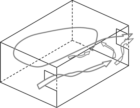
Schematic View - Room airflow dominated by jet

![Schematic - Room airflow -- a combination of jet and recirculation flow](media/image2384.png)

In Figure 133, the recirculation flow develops horizontally and the room airflow is dominated by the jet. In Figure 134, when buoyancy effects are important a more complex flow pattern develops. The recirculation flow moves vertically along its path and the outflow is a combination of jet and recirculation flow.

Implementation[LINK]

The model predicts representative air temperatures and airflow velocities in two regions of the flow: jet and recirculations. In addition a set of flow pattern related parameters are also predicted such as type of flow pattern (with or without recirculations), room length along the cross ventilation direction, inflow aperture area, and, for flow with recirculations the ratio between recirculation and inflow rate.

Structure of the implementation[LINK]

The calculation routine follows the following steps sequentially in every time step:

Identify the dominant aperture and obtain its area, width and inflow velocity.
Calculate room length and cross sectional area, check criteria .
Check whether recirculations are present in the flow, evaluate parameter C_L.
Predict relevant flow characteristics using expressions , , and .
If recirculations are present and all CV flow criteria are met, calculate recirculation flow temperature and surface mixed convection heat transfer coefficients.
Calculate jet region temperatures.
If the air temperature increase is above 1.5C or one of the CV flow criteria failed, perform a mixed flow calculation.

Outputs[LINK]

Representative airflow temperatures for the jet and recirculation regions are obtained by taking the average between predicted temperatures at the beginning and end of each stream:

Room Air Zone Jet Region Temperature [C] =

Room Air Zone Recirculation Region Temperature [C] =

In both cases T_J and T_R are the solutions of the system of differential equations shown in Equation(s) .

The outputs Room Air Zone Jet Region Average Air Velocity [m/s] and Room Air Zone Recirculation Region Average Air Velocity [m/s] are predicted using expressions and .

Nomenclature for Cross-Ventilation RoomAir Model[LINK]

Nomenclature for Cross-Ventilation RoomAir Model
Variable	Description
A*:	room non dimensional cross-section area ratio.
A_IN:	Inlet area (m²).
A_R:	Room cross section area (m²)
A_S:	Total room surface area (m²).
A_SL:	Shear layer heat transfer area (m²)
C_L:	Non-dimensional room aspect ratio (expression 1.18, chapter 1).
C_n:	correlation constant for correlation index “n”.
C_p:	Heat capacity of the air at constant pressure (J/(Kg.K)).
f:	Correlation function.
F:	Ventilation airflow rate (m³/s).
F_R:	flow rate in the recirculation region (m³/s).
H:	Room height (m).
h_F:	Surface averaged forced convection heat transfer coefficient.
h_FS:	Free stream heat transfer coefficient (W/(m²K)).
h_N:	Surface averaged natural convection heat transfer coefficient.
h_S:	Local surface heat transfer coefficient (W/(m²K)).
h_SL:	Shear layer heat transfer coefficient (W/(m²K)).
L_R:	Room length along the cross ventilation direction (m).
L*:	room non-dimensional length ratio.
M:	Momentum flux (N or J/m).
Q_Y=0:	Heat transfer in the shear layer mid plane (W).
R:	Non-dimensional recirculation flow ratio.
T(x):	Room air temperature, averaged in the YZ plane (C).
T_IN:	Average inlet airflow temperature (C).
T_J(x):	Temperature in the jet region, averaged in the YZ plane (C).
T_OUT:	Average temperature of the air leaving the room (K).
T_R:	Perfectly mixed room air temperature (C).
T_R(x):	Temperature in the section of the recirculation flow that is parallel to the jet region, averaged in the YZ plane (C).
T_W(r):	Temperature in the section of the recirculation that flows along the room walls, averaged in the YZ plane (C).
U_J:	average velocity in the room volume occupied by inlet jet flow (m/s).
U_R:	averaged velocity in a given region of the room that is being modeled (m/s).
U:	Characteristic velocity of the forced flow that “drives” the forced convection boundary layer.
W:	Room width (m).
W_IN:	width of the inlet aperture (m).
x:	Coordinate along the length of the boundary layer.
x_Outlet:	Location of the outlet along the room length (m).
T_J:	Temperature variation in the jet region (K).
T_R:	Temperature variation in the recirculation region (K).
T_SL:	Temperature variation in the shear layer region (K).
:	Air density (Kg/m³).
:	experimentally determined constant that scales mixing in the shear layer.

References[LINK]

Carrilho da Graca, G. 2003. Simplified models for heat transfer in rooms. Ph. D. Thesis, University of California, San Diego.

Kalema, T., Haapala, T. `995. Effect of interior heat transfer coefficients on thermal dynamics and energy consumption, Energy and Buildings 22 (2) pp. 101-113.

Aynsley, R.M., Melbourne, W., Vickery, B.J. 1977. Architectural Aerodynamics. Applied Science London.

Baturin, V. V. , Billington, N. S. 1972. Fundamentals of Industrial Ventilation, Franklin Book Company 1972, pp. 174-179.

Neiswanger, L., Johnson, G.A., Carey, V.P. 1987. An experimental study of high Raleigh number mixed convection in a rectangular enclosure with restricted inlet and outlet openings. Transactions of ASME, Vol. 109, 446-453.

Ohba, M., Irie, K., Kurabuchi, T. 2001. Study on airflow characteristics inside and outside a CVmodel, and ventilation flow rate using wind tunnel experiments. Journal of Wind Engineering and Industrial Aerodynamics, in press.

Chandra, S., Kerestecioglu, A.A. 1984. Heat transfer in naturally ventilated rooms data from full-scale measurements, ASHRAE Transactions, Volume 90, part 1b 211-224.

Altmayer, E.F., Gadgil, A.J., Bauman, F.S., Kammerud, R.C. Correlations for convective heat transfer from room surfaces. ASHRAE Transactions, No. 2764.

Spitler, J. D., Pedersen, C.O., Fisher, D.E. 1991. Interior Convective Heat Transfer in Buildings with Large Ventilative Flow Rates. ASHRAE Transactions, Vol. 97, Pt.1, pp. 505-515.

Awbi, H.B. & Hatton, A. 1999. Natural convection from heated room surfaces, Energy and Buildings, 30, 233-244.

Siebers, D. L., Schwind, R. G., Moffat, R. J. 1983. Experimental Mixed Convection Heat Transfer From a Large Vertical Surface in a Horizontal Flow. SAND 83-8225, Sandia National Laboratories, Livermore CA.

Awbi, H.B. & Hatton, A. 2000. Mixed convection from heated room surfaces, Energy and Buildings, 32, 153-166.

Bejan, A. 1994. Convection Heat Transfer 2nd ed, Wiley, USA.

Engineering Reference — EnergyPlus 8.0

Engineering Reference

Alternative Modeling Processes[LINK]

RoomAir Models[LINK]

References:[LINK]

User Defined RoomAir Temperatures[LINK]

One-Node Displacement Ventilation RoomAir Model[LINK]

References[LINK]

Three-Node Displacement Ventilation RoomAir Model[LINK]

Overview[LINK]

Displacement Ventilation[LINK]

Non-uniform zone models[LINK]

Model Description[LINK]

Single Plume Two Layer Model[LINK]

Multiple Plumes and Wall Heat Transfer[LINK]

Implementation[LINK]

Iterative procedure[LINK]

Step 1[LINK]

Step 3[LINK]

Mixed calculation[LINK]

Final calculations[LINK]

References[LINK]

Under-Floor Air Distribution Interior Zone Model[LINK]

Overview[LINK]

Underfloor air distribution systems[LINK]

Model Description[LINK]

Implementation[LINK]

Iterative procedure[LINK]

Step 1[LINK]

Step 2[LINK]

Mixed calculation[LINK]

Final calculations[LINK]

References[LINK]

Under-Floor Air Distribution Exterior Zone Model[LINK]

Overview[LINK]

Underfloor air distribution systems[LINK]

Model Description[LINK]

Implementation[LINK]

Iterative procedure[LINK]

Step 1[LINK]

Step 2[LINK]

Mixed calculation[LINK]

Final calculations[LINK]

References[LINK]

Cross Ventilation Room Air Model[LINK]

Overview[LINK]

Cross-Ventilation[LINK]

Recirculating flow[LINK]

Effects of recirculating flow in heat transfer[LINK]

Existing approaches[LINK]

Model Description[LINK]

Airflow pattern[LINK]

Recirculation Region Average Velocity[LINK]

Heat transfer in recirculating flows[LINK]

Heat transfer in a shear layer[LINK]

Predicting air temperature in the recirculation region of the flow[LINK]

Heat transfer in recirculating flows with internal gains[LINK]

Heat gains in the jet region[LINK]

Heat gains in the recirculation region[LINK]

Limitations of the model[LINK]

Implementation[LINK]

Structure of the implementation[LINK]

Outputs[LINK]

Nomenclature for Cross-Ventilation RoomAir Model[LINK]

References[LINK]